SIGNAL PROCESSING FOR NEXT-GEN SEQUENCING DATA
600 likes | 754 Vues
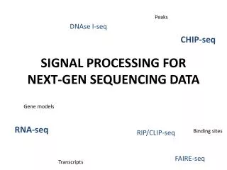
Peaks. DNAse I- seq. CHIP- seq. SIGNAL PROCESSING FOR NEXT-GEN SEQUENCING DATA. Gene models. RNA- seq. Binding sites. RIP/CLIP- seq. FAIRE- seq. Transcripts. The Power of Next-Gen Sequencing. Chromosome Conformation Capture. + More Experiments. DNA Genome Sequencing

SIGNAL PROCESSING FOR NEXT-GEN SEQUENCING DATA
E N D
Presentation Transcript
Peaks DNAse I-seq CHIP-seq SIGNAL PROCESSING FORNEXT-GEN SEQUENCING DATA Gene models RNA-seq Binding sites RIP/CLIP-seq FAIRE-seq Transcripts
The Power of Next-Gen Sequencing Chromosome Conformation Capture +More Experiments DNA Genome Sequencing Exome Sequencing DNAse I hypersensitivity CHART, CHirP, RAP CHIP CLIP, RIP CRAC PAR-CLIP iCLIP RNA RNA-seq Protein For more Seq technologies, see: http://liorpachter.wordpress.com/seq/
Next-Gen Sequencing as Signal Data • Map reads (red) to the genome. Whole pieces of DNA are black. • Count # of reads mapping to each DNA base signal Rozowskyet al. 2009 Nature Biotech
Outline • Read mapping: Creating signal map • Finding enriched regions • CHIP-seq: peaks of protein binding • RNA-seq: from enrichment to transcript quantification • Application: Predicting gene expression from transcription factor and histone modification binding Isoform 1 Isoform 2
Read mapping • Problem: match up to a billion short sequence reads to the genome • Need sequence alignment algorithm faster than BLAST Rozowskyet al. 2009 Nature Biotech
Read mapping (sequence alignment) • Dynamic programming • Optimal, but SLOW • BLAST • Searches primarily for close matches, still too slow for high throughput sequence read mapping • Read mapping • Only want very close matches, must be super fast
Index-based short read mappers • Similar to BLAST • Map all genomic locations of all possible short sequences in a hash table • Check if read subsequences map to adjacent locations in the genome, allowing for up to 1 or 2 mismatches. • Very memory intensive! Trapnell and Salzberg2009, Slide adapted from Ray Auerbach
Read Alignment using Burrows-Wheeler Transform • Used in Bowtie, the current most widely used read aligner • Described in Coursera course: Bioinformatics Algorithms (part 1, week 10) Trapnell and Salzberg2009, Slide adapted from Ray Auerbach
Read mapping issues • Multiple mapping • Unmapped reads due to sequencing errors • VERY computationally expensive • Remapping data from The Cancer Genome Atlas consortium would take 6 CPU years1 • Current methods use heuristics, and are not 100% accurate • These are open problems 1https://twitter.com/markgerstein/status/396658032169742336
transcription factor histone modification FINDing enriched regions: CHIP-seq data analysis Park 2009 Nature Reviews Genetics
CHIP-seq Intro • Determine locations of transcription factors and histone modifications. • The binding of these factors is what regulates whether genes get transcribed. Park 2009 Nature Reviews Genetics
CHIP-seq protocol DNA bound by histones and transcription factors Target protein of interest with Antibody Sequence DNA bound by protein of interest Park 2009 Nature Reviews Genetics
CHIP-seq Data # of sequence reads Chromosomal region Basic interpretation: Signal map to represents binding profile of protein to DNA How do we identify binding sites from CHIP-seq signal “peaks”? Park 2009 Nature Reviews Genetics
“Naïve” CHIP-seq analysis • Background assumption: all sequence reads map to random locations within the genome • Divide genome into bins, distribution of expected frequencies of reads/bin is described by the Poisson distribution. • Assign p-value based on Poisson distribution for each bin based on # of reads Rozowskyet al. 2009 Nature Biotech, Park 2009 Nature Reviews Genetics
Is a Poisson background reasonable for CHIP-seq data? • “Input” experiment: Do CHIP-seq using an antibody for a protein that doesn’t bind DNA • There are also “peaks” in the input! Park 2009 Nature Reviews Genetics
Is a Poisson background reasonable for CHIP-seq data? • “Input” is from a CHIP-seq experiment using an antibody for a non-DNA binding protein
Determining protein binding sites by comparing CHIP-seq data with input Candidate binding site identification Input normalization Input normalization/ bias correction Comparison of sample vs. input
Peakseq Rozowskyet al. 2009 Nature Biotech Gerstein Lab
Candidate binding site identification • Use Poisson distribution as background, as in the “naïve” analysis discussed earlier • Normalize read counts for mappability (uniqueness) of genomic regions • Use large bin size, finer resolution analysis later Rozowskyet al. 2009 Nature Biotech
Input normalization • Normalize based on slope of least squares regression line. Normalized reads = CHIP-seq reads/(slope*input reads) Rozowskyet al. 2009 Nature Biotech
Input normalization All data points Candidate peaks removed • Using regression based on all data points (including candidate peaks) is overly conservative. Rozowskyet al. 2009 Nature Biotech
Calling peaks vs. input • Binomial distribution • Each genomic region is like a coin • The combined number of reads is the # of times that the coin is flipped • Look for regions that are “weighted” toward sample, not input ENCODE NF-Kb CHIP-seq data
Multiple Hypothesis Correction • Millions of genomic bins expect many bins with p-value < 0.05! • How do we correct for this?
Multiple Hypothesis Correction • Bonferroni Correction • Multiply p-value by number of observations • Adjusts p-values expect up to 1 false positive • Very conservative
Multiple Hypothesis Correction • False discovery rate (FDR) • Expected number of false positives as a percentage of the total rejected null hypotheses • Expectation[false positives/(false positives+truepostives)] • q-value: maximum FDR at which null hypothesis is rejected. • Benjamini-Hochberg Correction • q-value = p-value*# of tests/rank
Many other CHIP-seq “peak”-callers Wilbanks EG, Facciotti MT (2010) Evaluation of Algorithm Performance in ChIP-Seq Peak Detection. PLoS ONE 5(7): e11471. doi:10.1371/journal.pone.0011471 http://www.plosone.org/article/info:doi/10.1371/journal.pone.0011471
CHIP-seq summary • Method to determine DNA binding sites of transcription factors or locations of histone modifications • Must normalize sequence reads to experimental input • Search for signal enrichment to find peaks • Peakseq: binomial test + Benjamini-Hochberg correction • Many other methods
RNA-seq • Searching for “peaks” not enough: • Are these “peaks” part of the same RNA molecule? • How much of the RNA is really there? Wang et alNature Reviews Genetics 2009
Background: RNA splicing • pre-mRNA must have introns spliced out before being translated into protein. • The final components of an mRNA are called exons intron exon
Background: alternative splicing • Alternative splicing leads to creation of multiple RNA isoforms, with different component exons. • Sometimes, exons can be retained, or intronscan be skipped. intron exon Isoform 1 Isoform 2
Simple quantification • Count reads overlapping annotations of known genes • Simplest method: Make composite model of all isoforms of gene • Quantification: Reads per kilobase per million reads (RPKM)
Isoform Quantification • Map reads to genome • How do we assign reads to overlapping transcripts?
Isoform Quantification • Simple method: only consider unique reads
Isoform Quantification • Simple method: only consider unique reads • Problem: what about the rest of the data?
Expectation Maximization Algorithm • Assign reads to isoforms to maximize likelihood of generating total pattern of observed reads. • 0. Initialize (expectation): Assign reads randomly to isoforms based on naïve (length normalized) probability of the read coming from that isoform (as opposed to other overlapping isoforms) LiorPachter 2011 ArXiv
Expectation Maximization Algorithm • 1. Maximization: Choose transcript abundances that maximize likelihood of the read distribution (Maximization). LiorPachter 2011 ArXiv
Expectation Maximization Algorithm • 2. Expectation: Reassign reads based on the new values for the relative quantities of the isoforms. LiorPachter 2011 ArXiv
Expectation Maximization Algorithm • 3. Continue expectation and maximization steps until isoform quantifications converge (it is a mathematical fact that this will happen). LiorPachter 2011 ArXiv
Detecting new transcripts • Search for “peaks”: • Reads that overlap splice junctionspeaks part of same transcript • Special sequencing techniques to find ends of transcripts • Still a major open area of research Wang et alNature Reviews Genetics 2009
RNA-Seq conclusions • RNA-Seq is a powerful tool to identify new transcribed regions of the genome and compare the RNA complements of different tissues. • Quantification harder than CHIP-seq because of RNA splicing • Expectation maximization algorithm can be useful for quantifying overlapping transcripts
RNA-seq Expression Correlation • Correlate expression between tissues Slide adapted from L Habegger
CHIP-seq signals of interacting proteins • Fos and Jun, which interact physically, have similar binding profiles at many genomic loci. Fos Jun Data from ENCODE Consortium, figure by me
Signal aggregation • Sum signals from all genomic locations of a certain type • Here: CHIP seq signal at fixed distances from protein binding motif Venters and Pugh Nature 2013
“Input” To what extent the gene expression levels are determined by TF binding/ HM modification? Histone modification TF Binding signal Predictive models Gene expression levels Relating gene expression with histone modification and TF binding signals “Output” Slide by Chao Cheng
Setting up the model TTS (transcription terminal site) TSS (transcription start site) Genek 1. Divide area around gene into bins according to distance to trascription start and end sites 80 40 1 120 81 121 160 4 … 41 ….44 Bin 120-81 (TTS-4kb to TTS) Bin 40-1 (TSS-4kb to TSS) Bin 121-160 (TTS to TTS+4kb) Bin 41-80 (TSS to TSS+4kb) Slide by Chao Cheng
Setting up the model TTS (transcription terminal site) TSS (transcription start site) Genek 2. Collect histone modification data for each bin, and for each gene 80 40 1 120 81 121 160 4 … 41 ….44 Bin 120-81 (TTS-4kb to TTS) Bin 40-1 (TSS-4kb to TSS) Bin 121-160 (TTS to TTS+4kb) Bin 41-80 (TSS to TSS+4kb) Chromatin features: Histone modifications Predictors ~10000 refseq genes HM1, 2, 3, …… …… Bin 1 Bin 2 Bin160 Slide by Chao Cheng
