Chapter 7 Implementation

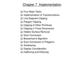
Chapter 7 Implementation • Four Major Tasks • Implementation of Transformations • Line-Segment Clipping • Polygon Clipping • Clipping of Other Primitives • Clipping in Three Dimensions • Hidden-Surface Removal • Scan Conversion • Bresenham’s Algorithm • Scan Conversion of Polygons • Antialiasing • Display Consideration • Halftoning and Dithering

Four Major Tasks • Modeling • produce geometric objects such as a set of vertices • Geometric Processing • 4 steps • Normalization (user coord  world coord  camera coord) • Clipping • Hidden-surface removal • Shading • determine which geometric objects appear on the display, and assign shade or color to these objects • Rasterization (Scan Conversion) • generate a set of pixel values for graphics primitives • Display • improve the quality of display (ex) jaggedness (aliasing) -> antialiasing

Four Major Tasks • Basic Implementation Strategies • object-oriented approach • for(each_object) render(object) • Figure 7.2 • pipelined rendering: implemented with special-purpose chips • image-oriented approach • for(each_pixel) assign_a_color(pixel) • require complex data structures <- which primitives affect which pixels • use coherence of pixels -> increamental algorithms

Implementation of Transformations • Coordinate Systems and Transformations • object (world) coordinate • eye (camera) coordinate • clip coordinate • normalized device coordinate (NDC) • window (screen) coordinate

Line-Segment Clipping (1) • Cohen-Sutherland Clipping • avoid intersection calculations, if possible • break up space into the nine regions • encode the line endpoints in outcode(b0b1b2b3) • reason on the basis of the outcodes • Let o1 = outcode(x1, y1) and o2 = outcode(x2, y2) for a line segment with endpoints (x1, y1), (x2, y2) • (o1 = o2 = 0): both endpoints are inside the clipping window [AB] • (o1 0, o2 = 0; or vice versa): one endpoint is inside the clipping window, the other is outside [CD] • (o1 & o2 0): both endpoints lie on the same outside side of the window [EF] • (o1 & o2= 0): both endpoints are outside, but on the outside of different edges of the window [GH,IJ]

Line-Segment Clipping (2) • Liang-Barsky Clipping • use the parametric form for lines: p1 = [x1, y1]T, p2 = [x2, y2]T • matrix form P(a) = (1 - a) p1 + a p2 (0 a 1) • scalar equations x(a) = (1 - a) x1 + a x2 y(a) = (1 - a) y1 + a y2 • find parameters a1a2a3a4 for the 4 points where the line intersects the extended sides of the window. • sort the parameters and determine the topological relationships 1 > a4 > a3 > a2 > a1 > 0 : clipped line segment [a2,a3] 1 > a4 > a2 > a3 > a1 > 0 : outside line segment

Line-Segment Clipping (3) • Intersection Computation • Cohen-Sutherland clipping • need floating-pointing number divisions: x = (y - h)/m • bisection method • Liang-Barsky clipping • use the value of four parameters • in the top of window: ymax = y1+a(y2-y1) • robust and faster the Cohen-Surtherland clipping

Polygon Clipping (1) • Nonconvex Polygon Clipping • may generate multiple clipped polygons from a polygon • treat the result of the clipper as a simple polygon • use only convex polygons, or divide (tessellate) a given polygon into a set of convex polygons

Polygon Clipping (2) • Sutherland-Hodgeman Polygon Clipping • applicable to convex polygons • pipeline clipping

Clipping of Other Primitives (1) • Bounding Boxes • bounding box (extent) of a polygon • the smallest rectangle, aligned with the window, that contains the polygon • use the information of bounding box for (many-sided) polygons to filter polygons

Clipping of Other Primitives (2) • Curves, Surfaces, and Texts • curves, surfaces • complicated to process them directly • approximate with line segments and planar polygons • texts • bitmap characters • done in the frame buffer without any geometric processing • stroke(outline) characters • defined standard primitives • processed by geometric processing through the standard viewing pipeline (cf) all-or-none • Clipping in the Frame Buffer • delay clipping until converted into screen coordinates • done in the frame buffer -> scissoring technique

Clipping in Three Dimensions • 3D Clipping Algorithms • Cohen-Sutherland • use 6-bit outcode in parallelepiped view volume • Liang-Barsky • add the parametric equation for z-axis z(a) = (1 - a)z1 + az2 • find 6 a values • Sutherland-Hodgeman • add extra two clippers for the z-axis components • extend 2D clipping algorithm to 3D environment -> clip lines or surfaces against surfaces p(a) = (1 - a)p1 + ap2 n•(p(a)- p0) = 0 -> a = n•(p0 - p1) / n•(p2 - p1)

Hidden-Surface Removal (1) • Hidden-Surface-Removal • remove those surfaces that should not be visible to the viewer • object-space approaches • order the surfaces of the objects in the scene such that drawing surfaces in a particular order provides the correct images • painter’s algorithm • image-space approaches • determine the relationship among objects on each projector (a ray that leaves the center of projection and passes through a pixel) • z-buffer algorithm • Back-Face Removal (Culling) • back faces are invisible • eliminate all back-facing polygons before applying hidden-surface-removal algorithm • find the angle  between the normal and the viewer • the polygon is facing forward if and only if -90    90 (i.e., cos 0) n • v 0 • glCullFace(GL_BACK)

Hidden-Surface Removal (2) • Z-Buffer Algorithm • easy to implement • z-buffer : keep depth information • process polygon by polygon as follows: • for each point on the polygon corresponding to the intersection of the polygon with a ray through a pixel, • compute and compare its distance for determining whether or not to update the pixel

Hidden-Surface Removal (3) • Painter’s Algorithm (Depth Sorting Method) • basic procedure • sort surfaces in order of decreasing depth • scan convert surfaces in order, starting with the surface of greatest depth • Figure 7.32

Hidden-Surface Removal (4) • Scan-Line Algorithm • rasterize the polygon scan line by scan line • determine the visible polygon by incremental depth calculation

Scan Conversion (1) • DDA (Digital Differential Analyzer) Algorithm • two endpoints (x1, y1), (x2, y2) m = (y2- y1)/(x2- x1) = y/x y = m when x is increased by 1 for (ix = x1; ix <= x2; ix++) { y += m; write_pixel(ix, round(y), line_color); } • high and low slope lines

Scan Conversion (2) • Bresenham’s Algorithm • d = a - b • if d is positive, the next pixel is in (i+3/2, j+1/2) • otherwise, the next pixel is in (i+3/2, j+3/2) • increamental processing dk : d at x = k + 1/2 xk = (k+1/2), yk : y value at xk dk+1 =dk-2y x + 2x(yk+1 - yk) if (dk > 0) dk+1 =dk-2y else dk+1 =dk-2y + 2x

Scan Conversion of Polygons (1) • Flood Fill Algorithm • two colors : background color, a foreground(drawing) color • the boundaries of a polygon are drawn in the foreground color • start from an inside point (x, y) flood_fill(int x, int y) { if (read_pixel(x, y) == Background_Color) { write_pixel(x, y, Foreground_Color); flood_fill(x - 1, y); flood_fill(x + 1, y); flood_fill(x, y - 1); flood_fill(x, y + 1); } }

Scan Conversion of Polygons (2) • Scan-Line Algorithm • find the spans(groups of continuous pixels) on each scan line • spans are determined by the set of intersections of polygons with scan lines • odd-even rule • testing for defining the inside of the polygon • odd-crossing : inside • even-crossing : outside • singularities

Antialiasing (1) • Aliasing • the distortion of information due to low-frequency sampling (undersampling) • jagged or stair-step appearance in raster image : digitization error • Antialiasing • methods to improve the appearance of displayed raster images

Antialiasing (2) • Antialiasing • area sampling -> applicable to spatial-domain ailiasing [F0756] • determine the pixel intensity by calculating the areas of overlap of each pixel with the object to be displayed • set each pixel intensity proportional to the area of overlap of the pixel with the finite-width line • supersampling -> applicable to time-domain aliasing [F0757] • sample object characteristics at a high resolution and display the results at a low resolution • obtain the pixel intensity information from multiple points that contribute to the overall intensity of a pixel

Display Consideration • Color Systems • difference in color systems: similar to different coordinate systems • C2 = M C1 , M: 3x3 color conversion matrix, determined from the literature or by experimentation • Gamma Correction • intensity -> perceived in a logarithmic manner log I = C0 + r log V • intensities should increase exponentially for uniform spaced brightness

Halftoning and Dithering • Halftoning • technique to simulate gray levels by creating patterns of black dots of varying size • Dithering • use digital halftone to simulate halftoning with fixed sized pixels

Chapter 7 Implementation