Neuro-symbolic programs for robots
Neuro-symbolic programs for robots. Ernesto Burattini*, Edoardo Datteri°, Guglielmo Tamburrini*. *Dipartimento di Scienze Fisiche, Università di Napoli “Federico II” °Dipartimento di Filosofia, Università di Pisa {ernb,datteri,tamburrini}@na.infn.it. NeSy'05


Neuro-symbolic programs for robots
E N D
Presentation Transcript
Neuro-symbolic programs for robots Ernesto Burattini*, Edoardo Datteri°, Guglielmo Tamburrini* *Dipartimento di Scienze Fisiche, Università di Napoli “Federico II” °Dipartimento di Filosofia, Università di Pisa {ernb,datteri,tamburrini}@na.infn.it NeSy'05 Neural-Symbolic Learning and Reasoning Workshop at IJCAI-05, Edinburgh, Scotland, August 1st, 2005
SUMMARY • Introduction to cNSBL • Limits of cNSBL • Fibred Neural Nets • The eNSBL language • An example • Concluding remarks and future work
A chief goal for robotics today: RECONCILING LOGICAL REASONING AND REACTIVE BEHAVIOR subproblems : 1 - how to perform inference on large systems of rules meeting temporal constraints 2 - how to combine sensory information, provided by sensors as continuous signals, with typically discrete rule processing.
1 - How to perform inference on large systems of rules meeting temporal constraints • We demonstrated* that mechanisms of monotonic and non-monotonic forward reasoning can be implemented and controlled using McCulloch and Pitts neurons. • We introduced a language cNSBL to represent these reasoning mechanisms. • cNSBL programs can be compiled and implemented on a parallel processor (FPGA). * [Burattini et al., 2000].
cNSBL building blocks - A literal L is represented by neural element Nli, - the negation of literal L is represented by another neural element N~li * We stipulate that the truth-value of each propositional literal L can be True (Nli is active), False (N~ liis active), or Undefined (Nli and N~ liare quiescent)**. * [Burattini et al., 2000]. **[von Neumann 1956].
Why three-valued propositions? • Epistemic (or even ontological) motivations: • robotic systems may be compelled to act even when the truth-value of some given sentence is undefined; • and the action to undertake when the truth-value of some given sentence is undefined may differ from actions the system would undertake if the sentence were either (known to be) true or (known to be) false.
p1 spc= n - a1,c p2 a2,c pc pn an,c - j sc =j - Qm = 1 pc Pj 1 cNSBL operators Let P={pi} (0 < i < n) and Q={qi}(0 < j < m) be sets of propositional literals (for some n, mN). Let P be the conjunction of the elements of P, and let Q be the disjunction of the elements of Q; let s be a literal. IMPLY(P, s) is intuitively interpreted as “IF the conjunction of literals P is true THEN s is true” UNLESS(P, Q, s) is intuitively interpreted as “IF the conjunction of literals P is true and the disjunction of literals Q is false or undefined THEN s is true”.
Two Examples • Traffic light example • Ethological example
Traffic light example Suppose that a robot has to cross the street. If there is a traffic-light then the robot crosses provided that the light is green, otherwise it waits. If there isn't a traffic-light at all, (the truth value for both green and not green is undefined) then the robot looks to the right and to the left in order to decide whether to cross the street or not. IMPLY( wish_to_cross G, cross) IMPLY( wish_to_cross G, not_cross) UNLESS( wish_to_cross, (G G), look_around)
Ethological example There are animals which pretend to be dead in order to deceive their predators. The behaviour of a “smart” predator may be descrided as follows: IMPLY( (there_is_a_prey prey_is_alive), eat_it) IMPLY( (there_is_a_prey prey_is_alive) , go_away) UNLESS( there_is_a_prey, (prey_is_alive prey_is_alive), verify)
library IEEE; use IEEE.std_logic_1164.all; entity neuron_ekb is port( clk, reset, edb : in std_logic; ekb : inout std_logic); end neuron_ekb; architecture SYN_USE_DEFA_ARCH_NAME of neuron_ekb is ………………. end SYN_USE_DEFA_ARCH_NAME; IMPLY(P, s) ……………… = 1 VHDL code neural network spc= n - a1,c p1 a2,c p2 pc VHDL compiler an,c Logic symbolic expressions cNSBL Formal neural network pn To peripheral devices inputs NSP (FPGA) Neurosymbolic compiler To symbolic interfaces FROM cNSBL TO FPGA IMPLEMENTATIONS
A behaviour-based system is represented in cNSBL as a layer* which is connected to sensory transduction and motor actuation mechanisms. At each time t (assuming discrete time), the state of the cNSBL layer is given by the truth-values of n propositional variables R={r1,…rn}. A finite set of cNSBL propositions (a cNSBL program) specifies how the values of some cNSBL variables in R at time t+1 depend on the value of the variables in R at time t. * [Aiello, Burattini, Tamburrini, 1995,1998]),
Subsumption architectures Avoid A Move_to_Goal G Motor M Wandering W Suppression of behaviours – competitive action selection mechanisms UNLESS(W, (G A), M) UNLESS(G, A, M) IMPLY(A, M)
Behavioural sequencing • IMPLY(a, backwardon) • IMPLY(backwardend, turnon) • IMPLY(turnend, forwardon) … backwardon backwardend turnon turnend forwardon a cNSBL layer motor actuation layer backward turn forward discrete actions
2 - How to combine sensory information, provided by sensors as continuous signals, with typically discrete rule processing. cNSBL is not sufficiently powerful to specify some familiar robotic behaviours and cooperative control functions. In the extended NSBL framework, behaviours are modelled as nets of threshold neurons (corresponding to sets of cNSBL rules), as fibred Neural Nets, (fNN for short, introduced in [d’Avila Garcez and Gabbay, 2004]), or as a combination of both. eNSBL is obtained by representing fNNs as real-valued variables, and by extending the semantics of IMPLY and UNLESS statements so as to admit real-valued variables as arguments.
Ii i Wj Fibred Neural Nets (fNN) A fibring function i from A to B maps the weights Wj of B to new values, depending on the values of Wj and on the input potential Ii of the neuron i in A; B is said to be embedded into A if i is a fibring function from A to B, and the output of neural unit i in A is given by the output of network B. The resulting network, composed of networks A and B, is said to be a fibred neural network . A Fibred Neural Network
eNSBL is obtained from cNSBL by allowing neurons to embed other neural networks via fibring functions. The output of neuron i is represented as an eNSBL real value (which we refer to by the superscript ‘e’). The statement IMPLY(a, be) is interpreted as “if a is true, then the network embedded in neuron b is enabled to compute a value for the eNSBL variable be”. No additional constraints are imposed on the other neurons of embedded networks.
As proved by d’Avila Garcez and Gabbay*, fibred neural networks can approximate any polynomial function to any desired degree of accuracy. Here, fNNs may be used to calculate attractive or repulsive potentials, or cooperative coordination among behaviours; and, for each fibred neural network Ni, the corresponding embedding neuron i enables the embedded network. d’Avila Garcez and Gabbay, 2004
Example of a potential field navigation mechanism based on eNSBL. An attractive (repulsive) potential is represented as a vector, whose direction points towards (away from) the goal, and whose magnitude is directly proportional to the distance between current point and goal or some sensory cue; A typical equation for the calculation of the repulsive vector magnitude is where x is the distance perceived by a range detector device and d is the maximum distance that the sensor can perceive. This potential field functions can be modeled by fNN
A sketch of the neural circuitry for calculating the potential fields This example includes six neurons, three of which (b, c, and m) embed nested fNNs. b calculates a repulsive potential, with sonar readings as input. c calculates an attractive potential, taking as input the local position of the robot and a map that represents the target position m blends the repulsive and attractive potentials by vectorial sum into one heading to be sent to the motors.
Each of the three computations is triggered by a cNSBL variable. The eNSBL program for this network is: IMPLY(p, be) IMPLY(q, ce) IMPLY(s, me)
Wp= 1 X0 p Wp= 1 p X1 b ’ = 0* (WK) = 0* (WK) ” = 1* (WK) = 1* (WK) K f(x) = x IY=i*WK*x x Y WK= i*1/d = IY*(WJ) =x/d*WJ*i J f(z) = z f(x) =1 m 1 WJ1=-1* =-1*x/d* i Z Iz =Wj1*1+WJ2*1/x=-1*x/d* i +1/x*d*x/d* i=1-x/d WJ2=d*=d*x/d* i f(x) = 1/x x ’ = IZ*(WH) th(Iz)=(1-x/d)*WH*Th(Iz)*i H f(x) =1 f(x) =x 1 = (1-x/d)*Th(1-x/d)*i Q WH=1*’
CONCLUSIONS • cNSBL is a significant tool for robotic BBS insofar as it: • enables one to meet reactive time responses • enables one to model competitive control • eNSBL extends cNSBL and • enables one to model cooperative control • enables one to combine connectionist and McCulloch & Pitts nets.
FUTURE WORK • Learning in hierarchically organized eNSBL nets • Wider logical repertoire for robotic control (modal logics, fragments of first order logic) • Implementation of eNSBL on FPGA processor.
REFERENCES • Aiello, A., Burattini, E., Tamburrini, G., 1995, "Purely neural, rule-based diagnostic systems. I, II”, International Journal of Intelligent Systems, Vol. 10, pp. 735-769. • Aiello, A., Burattini, E., Tamburrini, G., 1998, “Neural Networks and Rule-Based Systems”, in Leondes C. D. (ed.), Fuzzy Logic and Expert Systems Applications, Academic Press, Boston, MA. • Arbib, M., 1995, Schema Theory, in The Handbook of Brain Theory and neural Networks; M. Arbib ed., MIT press, Cambridge, MA, pp. 830-34 • Arkin R.C. - Behavior-based robotics - MIT Press – 1998 • Brooks, R.A., 1986, "A Robust Layered Control System for a Mobile Robot", IEEE Journal of Robotics and Automation, pp. 14-23 • Burattini, E., Datteri, E., Tamburrini, G., 2005, “Neuro-Symbolic Programs for Robots, IJCAI 2005 • Burattini, E., De Gregorio, M., Tamburrini, G., 2000, “NeuroSymbolic Processing: non-monotonic operators and their FPGA implementation”, in Proceedings of the Sixth Brazilian Symposium on Neural Networks (SBRN 2000), IEEE Press. • Burattini, E., Tamburrini, G., 1992, “A pseudo-neural system for hypothesis selection”, International Journal of Intelligent Systems, vol. 7, pp. 521-545. • d'Avila Garcez, A. S., Gabbay, D. M., 2004, “Fibring Neural Networks”, in Proceedings of 19th National Conference on Artificial Intelligence (AAAI 04), San Jose, California, USA, AAAI Press. • von Neumann, J.,1956, “Probabilistic logics and the synthesis of reliable organisms from unreliable components”, in C.E. Shannon, J. Mc Carthy (eds.), Automata Studies, Princeton U.P.
Wp= 1 Wp= 1 X0 X0 p p H J = IY*(WJ) =x/d*WJ*i Wp= 1 Wp= 1 p p X1 X1 b b ’ = IZ*(WH) th(Iz)=(1-x/d)*WH*Th(Iz)*i ” = 1* (WK) = i* (WK) Wp= 1 ’ = 0* (WK) = 0* (WK) ’ = 0* (WK) = 0* (WK) X0 p Iz =Wj1*1+WJ2*1/x=-1*x/d* i +1/x*d*x/d* i=1-x/d f(x) =1 ” = 1* (WK) = 1* (WK) ” = 1* (WK) = 1* (WK) Z 1 f(x) = x K K K f(x) = x f(x) = x ’ = 0* (WK) = 0* (WK) IY=i*WK*x IY=i*WK*x WJ1=-1* =-1*x/d* i IY=i*WK*x x x x Y Y Y f(z) = z WK= i*1/d WK= i*1/d x f(x) =1 f(x) =x WK= i*1/d f(x) = 1/x Wp= 1 X1 p b = IY*(WJ) =x/d*WJ*i = IY*(WJ) =x/d*WJ*i Q WJ2=d*=d*x/d* i J J 1 x f(z) = z f(z) = z f(x) =1 f(x) =1 WH=1*’ = (1-x/d)*Th(1-x/d)*i m m 1 1 WJ1=-1* =-1*x/d* i WJ1=-1* =-1*x/d* i Z Z Iz =Wj1*1+WJ2*1/x=-1*x/d* i +1/x*d*x/d* i=1-x/d Iz =Wj1*1+WJ2*1/x=-1*x/d* i +1/x*d*x/d* i=1-x/d WJ2=d*=d*x/d* i WJ2=d*=d*x/d* i = IY*(WJ) =x/d*WJ*i f(x) = 1/x f(x) = 1/x x x ’ = IZ*(WH) Th(Iz)=(1-x/d)*WH*Th(Iz)*i ’ = IZ*(WH) th(Iz)=(1-x/d)*WH*Th(Iz)*i ’ = IZ*(WH) th(Iz)=(1-x/d)*WH*Th(Iz)*i ” = 1* (WK) = 1* (WK) H H J f(x) =1 f(x) =1 f(x) =x f(x) =x 1 1 = (1-x/d)*Th(1-x/d)*i = (1-x/d)*Th(1-x/d)*i Q Q H m WH=1*’ WH=1*’
p1p2…pnpc spc= n - a1,c p1 a2,c p2 pc - j Variables are literals Conjunction of literals sc =j - an,c pn Pm pc Just one literal Pj = 1 1 IMPLY(P j, pc). UNLESS(Pj, Pm, pc)
c e a b d ¬d e b b d e d a DB d c a d a b a* KB c e b d ¬d a´ a´´ Input literals a, b, c, d, d, e a b d Ctrl d, d end d ¬d ctrl Output literals a, b, d Output a a b b d d Neural Forward Chaining Set of rules: b d e d a d c a d a b