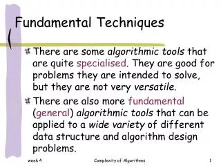
Fundamental Techniques
820 likes | 1.02k Vues
Fundamental Techniques. CS 5050 Chapter 5 Goal: review complexity analysis Talk of categories used to describe algorithms. Algorithmic Frameworks. Greedy Divide-and-conquer Discard-and-conquer Top-down Refinement Dynamic Programming Backtracking/Brute Force Branch-and-bound

Fundamental Techniques
E N D
Presentation Transcript
Fundamental Techniques CS 5050 Chapter 5 Goal: review complexity analysis Talk of categories used to describe algorithms.
Algorithmic Frameworks • Greedy • Divide-and-conquer • Discard-and-conquer • Top-down Refinement • Dynamic Programming • Backtracking/Brute Force • Branch-and-bound • Local Search (Heuristic)
Greedy Algorithms • Short-view, tactical approach to minimize the value of an objective function. • Eating whatever you want – no regard for health consequences or leaving some for others. • Example: Cheapest meal – beverage, main course, dessert, vegetable. Can we minimize cost by satisfying each category separately?
Greedy Algorithms • Solutions are often not global, but can be when problems satisfy the “greedy-choice” property • Example – Making change with US money to minimize number of coins; not true with other money systems. • Example – Knapsack problem. Given items weight and value. Want best value in knapsack within total weight limit. Cannot be done using greedy methods. Doesn’t have greedy choice property • It works best when applied to problems with the greedy-choice property: • a globally-optimal solution can always be found by a series of local improvements from a starting configuration.
The Greedy Method Technique • The greedy method is a general algorithm design paradigm, built on the following elements: • configurations: different choices, collections, or values to find • objective function: a score assigned to configurations, which we want to either maximize or minimize • Example: best path to take given I can only use {x1, … xn} locations? Does this have the greedy choice property? • Example: BST best binary search tree (best expected cost to find each entry). Does this have the greedy choice property? What if I always selected the root with the highest weight? (a:6, b:5, c:5 – should a be root?)
Making Change • Problem: A dollar amount to reach and a collection of coin amounts to use to get there. • Objective function: Minimize number of coins returned. • Greedy solution: Always return the largest value coin you can • Example 0: Coins are valued $1.00, $.50, $.25, $.10, $.05, $.01 • Example 1: Coins are valued $.32, $.08, $.01 • Has the greedy-choice property, since no amount over $.32 can be made with a minimum number of coins by omitting a $.32 coin (similarly for amounts over $.08, but under $.32). • There would never be a reason NOT to use the highest value coin. • Example 2: Coins are valued $.30, $.20, $.05, $.01 • Does not have greedy-choice property, since $.40 is best made with two $.20’s, but the greedy solution will pick three coins (which ones?)
The Knapsack Problem • Given: A set S of n items, with each item i having • bi - a positive benefit • wi - a positive weight • Goal: Choose items with maximum total benefit but with weight at most W. • Items are indivisible. • In this case, we let xi denote {1 if we take item, 0 otherwise} • Objective: maximize • Constraint:
The Knapsack Problem • Greedy will not work • Example: Knapsack of weight 10 Tent: weight 6, benefit 7 Food: weight 5, benefit 5 Clothing: weight 5, benefit 5 Tent has the (1) best total benefit and the (2) best benefit per pound but is not best to include.
The Fractional Knapsack Problem • Given: A set S of n items, with each item i having • bi - a positive benefit • wi - a positive weight • Goal: Choose items with maximum total benefit but with weight at most W. • If we are allowed to take fractional amounts, then this is the fractional knapsack problem. • In this case, we let xi denote the amount we take of item i • Objective: maximize • Constraint:
10 ml Example • Given: A set S of n items, with each item i having • bi - a positive benefit • wi - a positive weight • Goal: Choose items with maximum total benefit but with weight at most W. “knapsack” • Solution: • 1 ml of 5 • 2 ml of 3 • 6 ml of 4 • 1 ml of 2 Items: 1 2 3 4 5 Weight: 4 ml 8 ml 2 ml 6 ml 1 ml Benefit: $12 $32 $40 $30 $50 Value: 3 4 20 5 50 ($ per ml)
The Fractional Knapsack Algorithm • Greedy choice: Keep taking item with highest value (benefit to weight ratio) • Since • Run time: O(n log n). Why? Correctness: Suppose some choice k was wrong. Then we should have selected some amount of resource t. Let a be the smaller of the possible amounts of k and t. Since k has the higher value, a units of k must be worth more than a units of t. Hence, there was no mistake. AlgorithmfractionalKnapsack(S,W) Input:set S of items w/ benefit biand weight wi; max. weight WOutput:amount xi of each item i to maximize benefit with weight at most W for each item i in S xi 0 vi bi / wi{value} w 0{current weight} whilew < W remove item i with highest vi xi min{wi , W - w} w w + min{wi , W - w}
Task Scheduling • Given: a set T of n tasks, each having: • A start time, si • A finish time, fi (where si < fi) • Notice – the start and finish times are fixed!! • Goal: Perform all the tasks using a minimum number of “machines.” • How would you place task s so you didn’t have to rethink? Machine 3 Machine 2 Machine 1 1 2 3 4 5 6 7 8 9
Task Scheduling Algorithm • Greedy choice: consider tasks by their start time and use as few machines as possible with this order. • Run time: O(n log n). Why? • Must Sort • Correctness: Suppose there is a better schedule. • We can use k-1 machines • The algorithm uses k • Let i be first task scheduled on machine k • Machine i must conflict with k-1 other tasks • But that means there is no non-conflicting schedule using k-1 machines AlgorithmtaskSchedule(T) Input:set T of tasks w/ start time siand finish time fi Output:non-conflicting schedule with minimum number of machines m 0{no. of machines} whileT is not empty remove task i w/ smallest si if there’s a machine j for i then schedule i on machine j else m m +1 schedule i on machine m
Example • Given: a set T of n tasks, each having: • A start time, si • A finish time, fi (where si < fi) • [1,4], [1,3], [2,5], [3,7], [4,7], [6,9], [7,8] (ordered by start) • Goal: Perform all tasks on min. number of machines Machine 3 Machine 2 Machine 1 1 2 3 4 5 6 7 8 9
Divide-and-Conquer • Divide-and conquer is a general algorithm design paradigm: • Divide: divide the input data S in two or more disjoint subsets S1, S2, … • Recur: solve the subproblems recursively • Conquer: combine the solutions for S1,S2, …, into a solution for S • The base case for the recursion are subproblems of constant size • Analysis can be done using recurrence equations
Divide and Conquer Algorithms • Divide the problem into smaller subproblems - these are often equal sized • Eventually get to a base case • Examples – mergesort or quicksort • Generally recursive • Usually efficient, but sometimes not • For example, Fibonacci numbers – much duplicate work • Desirability depends on work in splitting/combining
Merge-Sort Review • Merge-sort on an input sequence S with n elements consists of three steps: • Divide: partition S into two sequences S1and S2 of about n/2 elements each • Recur: recursively sort S1and S2 • Conquer: merge S1and S2 into a unique sorted sequence AlgorithmmergeSort(S, C) Inputsequence S with n elements, comparator C Outputsequence S sorted • according to C ifS.size() > 1 (S1, S2)partition(S, n/2) mergeSort(S1, C) mergeSort(S2, C) Smerge(S1, S2)
Recurrence Equation Analysis • The conquer step of merge-sort consists of merging two sorted sequences, each with n/2 elements and implemented by means of a doubly linked list, takes at most bn steps, for some constant b. • Likewise, the basis case (n< 2) will take at b most steps. • Therefore, if we let T(n) denote the running time of merge-sort: • We can therefore analyze the running time of merge-sort by finding a closed form solution to the above equation. • That is, a solution that has T(n) only on the left-hand side.
Iterative Substitution(telescoping) • In the iterative substitution, or “plug-and-chug,” technique, we iteratively apply the recurrence equation to itself and see if we can find a pattern: • Note that base, T(n)=b, case occurs when 2i=n. That is, i = log n. • So, • Thus, T(n) is O(n log n).
Recursion tree – bn effort at each of log n levels. Show pictures of work (like we did in class) • Guess and test – eyeball, then attempt an inductive proof. If can’t prove, try something bigger/smaller. This is not a good way for beginning students.
The Recursion Tree • Draw the recursion tree for the recurrence relation and look for a pattern: Total time = bn + bn log n (last level plus all previous levels)
Master method (different from text)method of text can give tighter bounds • Of the form T(n) = c if n < d aT(n/b) +O(nk) if n >= d • a > bk then T(n) is O(n logb a ) • a = bk then T(n) is O(nk log n) • a < bk then T(n) is O(nk) • Can work this out on your own using telescoping and math skills.
Master Method, Example 1 • Example: • a=4 • b=2 • k=1 Case 1 says Solution: logba=2, so case 1 says T(n) is O(n2).
Master Method Example 2 • T(n) = 8T(n/2) +n2 • A=8 • B=2 • K = 2 • Case 3 8<4 so O(n2)
Master Method Example 3 • T(n) = T(n/2) +1 • A=1 • B=2 • K = 0 • Case 2 1=1 so O(log n)
Divide and ConquerWhen does it help? • Dividing the problem in half doesn’t always help. Example – canning peaches. There is no improvement in dividing the problem in half (and may actually be more work because of the overhead of setup and cleanup). • There are two ways dividing in half may help • As Jennie said – you may be able to throw part away. Like in a binary search, when the bad half is just discarded. • If the original complexity is greater than n and the “dividing the problem” or “putting back together” phase is linear, you can win. This is what happens in Quick sort. The division is linear, yet the work in a small subproblem is greater than linear. Say it is n2. Then the work becomes: (n/2)2 + (n/2)2 + O(n) = 2(n2/4) +n = n2/2 + n Thus in a single time of dividing in half, the coefficient on n2 is reduced If you do this recursively, the savings will be even greater.
Divide and ConquerInteger Multiplication • Algorithm: Multiply two n-bit integers I and J. • Divide step: Split I and J into high-order and low-order bits • We can then define I*J by multiplying the parts and adding: • So, T(n) = 4T(n/2) + n, which implies T(n) is O(n2). • But that is no better than the algorithm we learned in grade school. We have four multiplications each ¼ as big.
An Improved Integer Multiplication Algorithm • Algorithm: Multiply two n-bit integers I and J. • Divide step: Split I and J into high-order and low-order bits • Observe that there is a different way to multiply parts. • Suppose we played around with other choices and just happened to get the same answer but could reuse the same multiplications? • Suppose we tried to just subtract Ih and Il and subtract J the OPPOSITE way
An Improved Integer Multiplication Algorithm • Algorithm: Multiply two n-bit integers I and J. • Divide step: Split I and J into high-order and low-order bits • Observe that there is a different way to multiply parts: • So, T(n) = 3T(n/2) + n, which implies T(n) is O(nlog23), by the Master Theorem. • Thus, T(n) is O(n1.585).
Large Integer multiplication • Idea – How think of? You want a way of reducing the total number of pieces you need to compute. • Observe (Ih-Il)(Jl-Jh) = IhJl-IlJl – IhJh +IlJh • Key is for one multiply, get two terms we need if add in two terms we already have • So, instead of computing the four pieces shown earlier, we do this one multiplication to get two of the pieces we need!
Large Integer multiplication • IJ = IhJh2n +[(Ih-Il)(Jl-Jh)+IhJh+IlJl] 2n/2 + IlJl • Tada – three multiplications instead of four • by master formula O(n1.585) • a = 3 • b = 2 • k = 1
Try at seats!For Example Mult 75*53 I: 7 5 2 J: 5 3 -2 • 15 -4 Product 35*100 + 10(-4 + 35 + 15) + 15 75*53=3975
Matrix multiplication • Same idea Breaking up into four parts doesn’t help • Strassen’s algorithm: complicated patterns of sum/difference multiply reduce the number of subproblems to 7 (from 8) • Won’t go through details, as not much is learned from the struggle. • T(n) = 7T(n/2) + bn2 • Matrix multiplication is O(n2.808)
Homework • In using recursion to find best expected cost: Let expectedCost(a,b) return the integer representing the bestExpected cost in placing nodes a through b (where a,b are subscripts into order array of values to be placed) We need an auxiliary array to store the weights between subscripts IntexpectedCost(a,b) { if (a >b) return 0; if (a==b) return weight[a]; r = subscript of best root (trial and error to determine) cost1 = expectedCost(a,r-1) cost2 = expectedCost(r+1,b) theCost = weight[r] + cost1 + weight[a,r-1] + cost2 + weight[r+1,b] weight[a,b] = weight[r]+weight[a,r-1] + weight[r+1,b] return theCost; }
Homework • Notice how you repeatedly compute the same problems over and over again. • In memoizing, you record your results so you don’t have to repeat the problems. Store answers in bestCost[][]. Count the number of times you can just look up the bestCost rather than having to compute it.
Discard and Conquer • similar to divide and conquer • Discard and conquer requires only that we solve one of several subproblems • Corresponds to proof by cases • Binary search is an example • Finding kth smallest is an example (Quickselect)
Outline and Reading • Matrix Chain-Product (§5.3.1) • The General Technique (§5.3.2) • 0-1 Knapsack Problem (§5.3.3)
Dynamic Programming Algorithms • Reverse of divide and conquer, we build solutions from the base cases up • Avoids possible duplicate calls in the recursive solution • Implementation is usually iterative • Examples – Fibonacci series, Pascal triangle, making change with coins of different relatively prime denominations
Homework bestCost weight Notice we fill in main diagonal first. To compute bestCost[1,3] we look at [2,3] [1,1][3,3] [1,2]
Good Dynamic Programming Algorithm Attributes • Simple Subproblems • Subproblem Optimality: optimal solution consists of optimal subproblems. • Can you think of a real world example without subproblem optimality? Round trip discounts. • Subproblem Overlap (sharing)
The 0-1 Knapsack Problem • 0-1, means take item or leave it (no fractions) • Now given units which we can take or leave • Obvious solution of enumerating all subsets is Θ(2n) • Difficulty is in characterizing subproblems • Find best solution for first k units – no good, as optimal solution doesn’t build on earlier solutions • Find best solution, first k units within quantity limit • Either use previous best at this limit, or new item plus previous best at reduced limit – O(nW) • Pseudo-polynomial – as it depends on a parameter W, which is not part of other solutions.
Solve using recursion: int value[MAX]; // value of each item int weight[MAX]: // weight of each item //You can use item "item" or items with lower number //The maximum weight you can have is maxWeight // return the best value possible in the knapsack int bestValue(int item, int maxWeight) { if (item < 0) return 0; if (maxWeight < weight[item]) // current item can't be used, skip it return bestValue(item-1, maxWeight); useIt = bestValue(item-1, maxWeight - weight[item]) + value[item] dontUseIt = bestValue(item-1, maxWeight); return max (useIt, dontUseIt); }
Price per Pound • The constant `price-per-pound' knapsack problem is often called the subset sum problem, because given a set of numbers, we seek a subset that adds up to a specific target number, i.e. the capacity of our knapsack. • If we have a capacity of 10, consider a tree in which each level corresponds to considering each item (in order). Notice, in this simple example, about a third of the calls are duplicates.
We would need to store whether a specific weight could be achieved using only items 1-k. • possible[item][max] = given the current item (or earlier in the list) and max value, can you achieve max?
Consider the weights: 2, 2, 6,5,4 with limit of 10 • We could compute such a table in an iterative fashion:
Consider the weights: 2, 2, 6,5,4 with limit of 10 • We could compute such a table in an iterative fashion:
From the table • Can you tell HOW to fill the knapsack?
Let's compare the two strategies: • Normal/forgetful: wait until you are asked for a value before computing it. You may have to do some things twice, but you will never do anything you don't need. • Compulsive/elephant: you do everything before you are asked to do it. You may compute things you never need, but you will never compute anything twice (as you never forget). • Which is better? At first it seems better to wait until you need something, but in large recursions, almost everything is needed somewhere and many things are computed LOTS of times.