Radio Astronomy
Radio Astronomy. ASTR 3010 Lecture 25. Intro to Radio Astronomy Concepts - Amplifiers - Mixers (down-conversion) - Principles of Radar - Radio Astronomy basics: System temperature, Receiver temperature Brightness temperature,

Radio Astronomy
E N D
Presentation Transcript
Radio Astronomy ASTR 3010 Lecture 25
Intro to Radio Astronomy • Concepts • - Amplifiers • - Mixers (down-conversion) • - Principles of Radar • - Radio Astronomy basics: • System temperature, Receiver temperature • Brightness temperature, • The beam (q = l / D) [ its usually BIG] • Interferometry (c.f. the Very Large Array – VLA) • Aperture synthesis
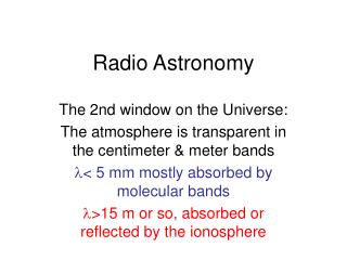
History of Radio Astronomy • (the second window on the Universe) • 1929 - Karl Jansky (Bell Telephone Labs) • 1030s - Grote Reber • 1940s - WWII, radar • - 21 cm (Jan Oort etc.) • 1950s - Early single dish & interferometry • - `radio stars’, first map of Milky Way • - Cambridge surveys (3C etc) • 1960s - quasars, pulsars, CMB, radar, VLBI • aperture synthesis, molecules, masers (cm) • 1970s - CO, molecular clouds, astro-chemistry (mm) • 1980s /90s – CMB anisotropy, (sub-mm)
Optical and Radio can be done from the ground! NRAO/AUI/NSF
Radio Telescope Optical Telescope Nowadays, there are more similarities between optical and radio telescopes than ever before. NRAO/AUI/NSF
Outline • A Simple Heterodyne Receiver System • mixers and amplification • Observing in the Radio • resolution • brightness temperature • Radio Interferometry • Aperture synthesis
Mixing: Adding waves together Freflect = f trans + / - Df f trans Df = 1850 Hz
Mixers A mixer takes two inputs: the signal and a local oscillator (LO). The mixer outputs the sum and difference frequencies. In radio astronomy, we usually filter out the high frequency (sum) component. local oscillator signal in LO w1 w2 signal out w1+w2 and w1-w2
mixed signal Mixers LO signal original signal 0 Hz frequency
mixed signal Mixers The negative frequencies in the difference appear the same as a positive frequency. To avoid this, we can use “Single Sideband Mixers” (SSBs) which eliminate the negative frequency components. LO signal original signal 0 Hz frequency
W-band (94 GHz, 4 mm) amplifier
filter A Simple Heterodyne Receiver signal @ 1420 MHz 1570 MHz receiver horn LO low noise amplifier 1420 MHz 150 MHz + + tunable filter Analog-to-Digital Converter Computer outputs a power spectrum tunable LO ~150 MHz
Observing in the Radio I • We get frequency and phase information, but not position on the sky • 2D detector • A CCD is also a 2D detector (we get x & y position)
Observing in the Radio II:Typical Beamsize (Resolution) • i.e. The BURAO 21 cm horn (D ~ 1 m)
Observing in the Radio II • i.e. The NRAO GBT (D ~ 100 m) at 21cm = 1.420 GHz at 0.3 cm = 100 GHz
Observing in the Radio II • i.e. The Arecibo Telescope (D ~ 300 m) at 21cm = 1.420 GHz at 0.3 cm = 100 GHz
Observing in the Radio III:Brightness Temperature Flux: erg s-1 sr-1 cm-2 Hz-1 (1023 Jy) Bu(T): erg s-1 sr-1 cm-2 Hz-1 (1023 Jy) We can use temperature as a proxy for flux (Jy) Conveniently, most radio signals have hu/kT << 1, so we can use the Raleigh-Jeans approximation Bu(T) = 2kT/l2 Thus, flux is linear with temperature
Antenna Temperature TB = Ful2/2k • Brightness temperature (TB) gives the surface temperature of the source (if it’s a thermal spectrum) • Antenna Temperature (TA): if the antenna beam is larger than the source, it will see the source and some sky background, in which case TA is less than TB • Noise in the system is characterized by the system temperature (Tsys) • i.e. you want your system temperature (especially in the first amp) to be low TA ~ TBWs/Wb
Radio Interferometry to source positional phase delay Q Q + East
Two Dish Interferometry • The fringe pattern as a function of time gives the East-West (RA) position of the object • Also think of the interferometer as painting a fringe pattern on the sky • the source moves through this pattern, changing the amplitude as it goes
Aperture Synthesis • A two dish interferometer only gives information on the E-W (RA) structure of a source • To get 2D information, we want to use several dishes spread out over two dimensions on the ground
Radio Telescope Arrays The VLA: An array of 27 antennas with 25 meter apertures maximum baseline: 36 km 75 Mhz to 43 GHz
Radio Telescope Arrays ALMA: An array of 64 antennas with 12 meter apertures maximum baseline: 10 km 35 GHz to 850 GHz
The U-V Plane • Think of an array as a partially filled aperture • the point source function (PSF) will have complicated structure (not an airy disk) • the U-V plane shows what part of the aperture is filled by a telescope • this changes with time as the object rises and sets • a long exposure will have a better PSF because there is better U-V plane coverage (closer to a filled aperture)
The U-V plane a snapshot of the U-V plane (VLBA) U-V coverage in a horizon to horizon exposure
Point Spread Function The dirty beam : the diffraction pattern of the array
Examples of weighting Dirty Beams: A snapshot (few min) Full 10 hrs VLA+VLBA+GBT
Image Deconvolution • Interferometers have nasty PSFs • To get a good image we “deconvolve” the image with the PSF • we know the PSF from the UV plane coverage • computer programs take a PSF pattern in the image and replace it with a point • the image becomes a collection of point sources
UV Plane Coverage and PSF images from a presentation by Tim Cornwell (given at NRAO SISS 2002)
UV Plane Coverage and PSF images from a presentation by Tim Cornwell (given at NRAO SISS 2002)
Image Deconvolution images from a presentation by Tim Cornwell (given at NRAO SISS 2002)
What emits radio waves? NRAO/AUI/NSF
Recipe for Radio Waves 1. Hot Gases NRAO/AUI/NSF
Electron accelerates as it passes near a proton. EM waves are released NRAO/AUI/NSF
Recipe for Radio Waves 2. Atomic and molecular transitions (spectral lines) NRAO/AUI/NSF
Gas Spectra Neon Sodium 656 nm 434 nm 486 nm Hydrogen NRAO/AUI/NSF
Electron accelerates to a lower energy state NRAO/AUI/NSF
Recipe for Radio Waves 3. Electrons and magnetic fields NRAO/AUI/NSF
Electrons accelerate around magnetic field lines NRAO/AUI/NSF