BA 187 – International Trade

1. BA 187 – International Trade Increasing Returns to Scale, Imperfect Competition & Trade

2. Economies of Scale & Market Structure • Increasing Returns to Scale (IRS) means that equal proportionate increase in inputs to production results in a more than equal proportionate change in output. • This implies cost per unit for output falls as output rises. • Two ways for this to occur: • External Economies to Scale • When cost per unit for output depends on size of the industry but not on the size of any one firm. (Think knowledge spillovers.) • Typically results in industry of many small firms acting as perfect competitors. (Think Silicon Valley, Multi-media Gulch, etc.) • Internal Economies of Scale • When cost per unit for output depends on the size of the individual firm but not necessarily on the size of the industry. (Think Natural Monopoly) • Typically results in advantage to few, large firms acting in imperfectly competitive manner. (Think Regulated Utilities, Microsoft, etc)

3. 2. In autarky, nations produce & consume at point A. 3. If each nation specializes in one of the goods and then trades to reach pt. E, both achieve higher utility. QY E UTrade A UAut QX PPF & Gains to Trade with RS 1. Assume PPF same for both nations & exhibits Increasing Returns to Scale. This means PPF is bowed inward towards origin. Good Y 4. Pattern of trade is indeterminate, either nation can specialize in either good. PPF with IRS Good X

4. 2. Assume that international terms of trade given. 3. Pattern of trade is technologically indeterminate, either nation can specialize in either good. 4. Nation is not indifferent between which good it produces. Will want to specialize in Good Y, as this results in highest utility. 5. Still mutual gains from trade but now strategic. E1 U1Trade E2 U2Trade Strategic Trade with IRS 1. Assume PPF same for both nations & exhibits IRS. Good Y QY PPF QX Good X

5. Older Approaches to Trade Patterns Product Cycle and Linder Demand Theories

6. Product Cycle Models • Based on presumption that introduction of new product conveys temporary monopoly in market. • New product requires highly skilled labor to produce • As product matures, it becomes standardized or can be imitated. • Comparative advantage shifts from innovating nation to nations with cheap labor. • Technological Gap model emphasizes time lag in imitation. • Product Cycle model emphasizes standardization process. Stage I: New Product Phase – Produced/consumed in innovating country only. Stage II: Product Growth Phase – Rising demand at home & abroad leads to exports from innovating country. Stage III: Product Maturity Phase – Product standardized, prod’n licensed to others. Stage IV: Imitation I Phase – Imitating country undersells originator in ROW. Stage V: Imitation II Phase – Imitating country undersells in originator’s market.

7. Consump. Exports Innovating Country Imports Prod’n Prod’n Imitating Country Exports Consump. Imports The Product Cycle Model Quantity Stage I Stage II Stage III Stage IV Stage V Time

8. Dates of Product Introduction & Characteristics of Industry 1970-1979 Date of Product Introduction Source: Thorelli & Burnett, “The Nature of Product Life Cycle for Industrial Goods Business”

9. Linder Demand Theory • Linder Theory focuses on role of demand, rather than supply, on trade patterns. • Assumes consumers’ tastes depend on their income levels. • A nation’s income level yields pattern of demand for goods. • The nation’s produce types of goods demanded within country, hence nation’s production reflects its income level. • Trade between countries occurs in goods for which there is overlapping demand, i.e. consumers in both countries have a demand for these particular items. • Implies that trade in certain goods should be more intense between countries with similar per capita income than between countries with dissimilar per capita incomes. • Consistent with product cycle model. • Consistent with empirical evidence generally & for manufactures in particular.

10. Per-Capita Income Demand Patterns Source: World Bank,World Bank Development Report, 1990

11. Linder & Intra-Industry Trade • Linder theory does not identify the direction in which any good flows. • In fact, a good might be traded in both directions. • This was not possible in previous models. • Intra-Industry trade: • Occurs when country imports and exports items in the same product classification. • Linder predicts this trade should be greatest between countries with similar per capita income levels. • Why Intra-industry trade? • Product Differentiation plus IRS can lead to each country specializing in particular variants for the joint “mass market”.

12. Intra-Industry Trade • Index of Intra-Industry Trade IIIT = 1 – |X-M|/(X+M) • No IIT then IIIT = 0, All IIT then IIIT = 1.0 • Why Intra-Industry Trade in an Industry? • Product Differentiation. • Transport Costs and Geographical Location. • Dynamic Economies of Scale (2+ versions of product). • Mismeasurement due to degree of product aggregation. • Differing Income Distributions within Countries.

13. New Approaches to Trade I IRS, Imperfect Competition and Intra-Industry Trade

14. Imperfect Competition • Pure Monopoly: • Firm faces no competition, faces downward-sloping Demand Curve. • Maximizes profit by setting Quantity to ensure: Marginal Revenue = MR = MC = Marginal Cost • Monopolistic Competition: • A-1: Each firm differentiates its product from that of rival firms. • A-2: Each firm takes rivals’ prices as given in setting own price. • Result: Each firm acts like a monopolist in pricing (MR = MC), even though each faces competition from many rivals. • Special case of oligopoly: • Market structures where firms have interdependent pricing decisions. • Ignoring opportunities for collusive behavior between firms. • Also ignoring opportunities for strategic behavior between firms.

15. 2. In SR number of firms fixed, each with produces differentiated product. 3. Each sets MR=MC to determine output level. 4. In SR all firms earn positive economic profits. Implies will have entry into industry. P ProfitSR AC DSR MRSR QMCSR SR Monopolistic Competition 1. Fixed Costs generate IRS for each firm. Cost, C and Price, P AC MC Quantity, Q

16. 1. Entry by new firms pushes down Demand Curve for each firm to DLR. 2. Entry continues until pushes DLR tangent to AC. 3. In LR equilibrium, each firm earns zero economic profits. More firms & more types of goods. P=AC DSR DLR MRSR MRLR QMCLR LR Monopolistic Competition Cost, C and Price, P AC MC Quantity, Q

17. The Krugman Model - Details • IRS at firm level due to fixed costs. • Firm-level costs: C = F + cQ or AC = F/Q + c • Firms produce differentiated goods with market structure that of monopolistic competition. • Firm-level Demand: Q = S[1/n – b(P-Pbar)] • Where S = Industry sales, Pbar= Competitor’s Price, n = #firms. • Industry-level costs (CC Curve): • AC = F/Q + c = F/(S/n) + c = n xF/S + c • More firms in the industry, the higher is the average cost. • Industry-level Price (PP Curve): • Set MR = P – Q/(S x b) = c or P = c + 1/(b x n) • More firms in the industry, the lower the price each firm charges. • Equilibrium: • CC and PP Curves intersect at zero-profit # of firms in industry

18. 1. Fixed Costs imply upward- sloping CC Curve. 2. Monopolistic competition implies downward-sloping PP Curve. AC2 CC 3. With n1 in industry, each firm makes +ve profits, entry occurs. P1 4. With n2 in industry, each firm makes -ve profits, exit occurs. P* =AC 5. Only at n* firms in the industry does each firm make zero profits, no entry or exit occurs. AC1 P2 PP n1 n* n2 The Krugman Model - Diagram Cost, C and Price, P Number of Firms, n

19. 1. Introduction of trade increases size of market. Result is lower CC Curve for any given level of n. CCTrade 2. More firms in market after trade, i.e. greater variety of goods. 3. In addition, lower AC and so Price for goods after trade. P1 =AC1 n1 Trade & the Krugman Model Cost, C and Price, P CC P0 =AC0 PP n0 Number of Firms, n

20. Intra-Industry Trade U.S. Imports/Exports of Auto Parts, Engines, & Bodies (Millions of $) Source: R.B. Cohen, Trade Policy in the 1980’s, IIE

21. Product Differentiation & Trade • With IRS technologies, trade & gains from trade can arise even if both economies identical. (Non-comparative advantage trade) • Several sources for gains from trade. Expansion of IRS sector leads to pro-competitive gains: profit effect and decreasing average cost effect. • Gains from trade may be captured as increased product diversity or lower average costs or both. Krugman model is example of where both occur together. • Trade based on scale economies may drive factor prices farther apart in the two countries. Also make it more likely, however, that all factors gain from trade.

22. New Approaches to Trade II Price-Discriminating Monopolists and Dumping

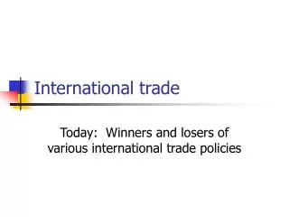
23. 1. Domestic Monopolist produces at MR=MC, (P0, Q0). 2. Assume can export output as price-taker at Pint =MRInt 3. Monopolist will equate MR across markets to allocate total output so as to maximize profits. 4. Result is that PHome higher than PInt, i.e. firm is “unfairly” dumping output in foreign market. PHome P0 PInt DInt = MRInt Q0 QHome QExports Total Q Monopoly and “Dumping” Cost, C and Price, P MC DHome MRHome Quantity, Q

24. 2. Will determine price/quantity in each market as MC =MR1 = MR2. 3. Result will be different prices in each market depending on demand conditions. P1 P2 D2 D1 MR2 MR1 Q1 Q2 Price Discriminating Monopolist 1. Assume Price-discriminating Monopolist with constant MC across markets. Cost, C and Price, P Cost, C and Price, P Market 1 Market 2 MC MC Quantity, Q Quantity, Q

25. New Approaches to Trade III External Economies of Scale and Trade

26. Sources of External Economies • External Economies to Scale occur at the level of the industry, rather than the individual firm. • Sources of External Economies • Clustering of Specialized Suppliers. • Localized industrial cluster of firms collectively create market large enough to support specialized equipment or support. • Pool for Specialized Labor. • Localized industrial cluster collectively create & support market for specialized labor. Benefits both labor & firms. • Knowledge Spillovers. • Localized industrial cluster of firms create informal exchange of ideas and knowledge for innovation.

27. 2. Developed Country (DC) initial producer of Good at Q0 and Pw = ACDC. 3. Less Developed Country (LDC) tries to enter with lower AC Curve. Unable to because cannot compete when denied scale effects of prod’n (Cost = C0 > Pw). C0 PW ACDC ACLDC Q0 External Economies & Specialization 1. Strong External Economies tend to reinforce existing patterns of IIT regardless of initial source. Cost, C and Price, P DWorld Quantity, Q

28. 2. Prohibitive tariff or quota closes LDC market. LDC producers face DLDC , produce to meet demand. 3. Domestic producers reach ACLDC = PLDC < Pw. Can now undersell DC producers on world market. PLDC DLDC Infant Industry Argument 1. LDC may try to protect its industry from ROW exports to gain scale effects in prod’n. Cost, C and Price, P C0 PW ACDC ACLDC DWorld Q0 Quantity, Q

29. 2. Learning Curves, LC, reflect cost saving from cumulative output learning effects. 3. Again, if DC is first in industry, cost savings from learning will dominate lower LCLDC. C0 PW LCDC LCLDC Q0 Dynamic Scale Economies 1. Strong Dynamic Learning effects reinforce existing patterns of IIT. Cost, C and Price, P DWorld Quantity, Q

30. Summary of Scale Effects on Trade Patterns

31. Empirical Summary of IRS Models • Gains from IRS occur in addition to gains from comparative advantage. Theories are thus complementary to Standard Trade model results. • Pattern of specialization, and thus trade patterns, inherently arbitrary. Possibly dependent on historical factors, open to strategic interventions (first mover advantage) to capture highest welfare effects. • IRS models offer more possibilities for gains from trade. • Empirical evidence indicates IRS important determinant of trade flows for countries size of Canada or Western European nations. Primarily rationalization of manufacturing. • Increased mobility of factors of prod’n (mostly capital) suggests comparative advantage models increasingly less important.