Autocorrelation, Box Jenkins or ARIMA Forecasting
Autocorrelation, Box Jenkins or ARIMA Forecasting. Autocorrelation and the Durbin-Watson Test.

Autocorrelation, Box Jenkins or ARIMA Forecasting
E N D
Presentation Transcript
Autocorrelation, Box Jenkins or ARIMA Forecasting
Autocorrelation and the Durbin-Watson Test An autocorrelation is a correlation of the values of a variable with values of the same variable lagged one or more periods back. Consequences of autocorrelation include inaccurate estimates of variances and inaccurate predictions. Lagged Residuals ii i-1 i-2 i-3 i-4 1 1.0 * * * * 2 0.0 1.0 * * * 3 -1.0 0.0 1.0 * * 4 2.0 -1.0 0.0 1.0 * 5 3.0 2.0 -1.0 0.0 1.0 6 -2.0 3.0 2.0 -1.0 0.0 7 1.0 -2.0 3.0 2.0 -1.0 8 1.5 1.0 -2.0 3.0 2.0 9 1.0 1.5 1.0 -2.0 3.0 10 -2.5 1.0 1.5 1.0 -2.0 The Durbin-Watson test (first-order autocorrelation): H0: 1 = 0 H1: 0 The Durbin-Watson test statistic:
DW d Test 4 Steps Step 1: Estimate And obtain the residuals Step 2: Compute the DW d test statistic Step 3: Obtain dL and dU: the lower and upper points from the Durbin-Watson tables
Critical Points of the Durbin-Watson Statistic: =0.05, n= Sample Size, k = Numberof Independent Variables k = 1 k = 2 k = 3 k = 4 k = 5 n dL dU dL dU dL dU dL dU dL dU 15 1.08 1.36 0.95 1.54 0.82 1.75 0.69 1.97 0.56 2.21 16 1.10 1.37 0.98 1.54 0.86 1.73 0.74 1.93 0.62 2.15 17 1.13 1.38 1.02 1.54 0.90 1.71 0.78 1.90 0.67 2.10 18 1.16 1.39 1.05 1.53 0.93 1.69 0.82 1.87 0.71 2.06 . . . . . . . . . . . . . . . . . . 65 1.57 1.63 1.54 1.66 1.50 1.70 1.47 1.73 1.44 1.77 70 1.58 1.64 1.55 1.67 1.52 1.70 1.49 1.74 1.46 1.77 75 1.60 1.65 1.57 1.68 1.54 1.71 1.51 1.74 1.49 1.77 80 1.61 1.66 1.59 1.69 1.56 1.72 1.53 1.74 1.51 1.77 85 1.62 1.67 1.60 1.70 1.57 1.72 1.55 1.75 1.52 1.77 90 1.63 1.68 1.61 1.70 1.59 1.73 1.57 1.75 1.54 1.78 95 1.64 1.69 1.62 1.71 1.60 1.73 1.58 1.75 1.56 1.78 100 1.65 1.69 1.63 1.72 1.61 1.74 1.59 1.76 1.57 1.78
Durbin-Watson Test for Autocorrelation: An Example The Banner Rock Company manufactures and markets its own rocking chair. The company developed special rocker for senior citizens which it advertises extensively on TV. Banner’s market for the special chair is the Carolinas, Florida and Arizona, areas where there are many senior citizens and retired people The president of Banner Rocker is studying the association between his advertising expense (X) and the number of rockers sold over the last 20 months (Y). He collected the following data. He would like to use the model to forecast sales, based on the amount spent on advertising, but is concerned that because he gathered these data over consecutive months that there might be problems of autocorrelation.
Durbin-Watson Test for Autocorrelation: An Example • Step 1: Generate the regression equation
Durbin-Watson Test for Autocorrelation: An Example • The resulting equation is: Ŷ = - 43.802 + 35.95X • The coefficient (r) is 0.828 • The coefficient of determination (r2) is 68.5% • There is a strong, positive association between sales and advertising • Is there potential problem with autocorrelation?
Durbin-Watson Test for Autocorrelation: An Example =-43.802+35.95*C3 =(E4-F4)^2 =E4^2 =B3-D3 =E3
Reject H0 Positive Autocorrelation Fail to reject H0 No Autocorrelation Inconclusive dl=1.20 du=1.41 Durbin-Watson Test for Autocorrelation: An Example • Hypothesis Test: H0: No residual correlation (ρ = 0) H1: Positive residual correlation (ρ > 0) • Critical values for d given α=0.5, n=20, k=1 dl=1.20 du=1.41
All stationary time series can be modeled as AR or MA or ARMA models A stationary time series is one with constant mean ( ) and constant variance. Stationary time series are often called mean reverting series—that in the long run the mean does not change (cycles will always die out). If a time series is not stationary it is often possible to make it stationary by using fairly simple transformations
Nonstationary Time series • Linear trend • Nonlinear trend • Multiplicative seasonality
How to make them stationary • Linear trend • Take non-seasonal difference. What is left over will be stationary AR, MA or ARMA • Nonlinear trend • Exponential growth • Take logs – this makes the trend linear • Take non--seasonal difference • Non exponential growth ? Take logs • Multiplicative seasonality often occurs when growth is exponential.
Identification • What does it take to make the time series stationary? • Is the stationary model AR, MA, ARMA • If AR(p) how big is p? • If MA(q) how big is q? • If ARMA(p,q) what are p and q?
ARMA models • If you can’t easily tell if the model is an AR or a MA, assume it is an ARMA model.
Box-Jenkins Method First of all, the analyst identifies a tentative model considering the nature of the past data. This tentative model and the data are entered in the computer. The Box-Jenkins program then gives the values of the parameters included in the model. A diagnostic check is then conducted to find out whether the model gives an adequate description of the data. If the model satisfies the analyst in this respect, then it is used to make the forecast.