The Box-Jenkins (ARIMA) Methodology
1.06k likes | 2.96k Vues
The Box-Jenkins (ARIMA) Methodology. ARIMA Models ( time series modeling ). A uto R egressive I ntegrated M oving A verage (ARIMA) models model stationary as well as nonstationary data do not involve independent variables in their construction

The Box-Jenkins (ARIMA) Methodology
E N D
Presentation Transcript
ARIMA Models(time series modeling) • AutoRegressive Integrated Moving Average (ARIMA) models • model stationary as well as nonstationary data • do not involve independent variables in their construction • rely heavily on autocorrelation (and partial autocorrelation) patterns in the data • aka “Box - Jenkins Methodology”
ARIMA Models • ARIMA models are designated by the level of autoregression, integration, and moving averages • Does not assume any pattern … uses an iterative approach of identifying a model • The model“Fits” if residuals are generally small, randomly distributed, and in general, contain no useful info
ARIMA Notation • ( AR I MA ) | | | p d q • Where • p = order of auto-regression (rare>2) • d= order of integration (differencing) • q= order of moving average (rare>2)
ARIMA Postulate a general class of models Identify Model to be considered Usemodel for Forecasting Estimate Parameters Check – Is the model Adequate ?? YES NO
The general (AR) model…for pth-order autoregressive model • Yt=dependent variable at time t • Yt-1, Yt-2, …Yt-p =responses in previous time periods … play the role of independent variables • s = coefficients to be estimated Appropriate for stationary time series
AR( ) • For auto-regresssive models, forecasts depend on observed values in previous time periods • AR(2) forecast of next depends on observations from previous 2 periods • AR(3) forecast of next depends on observations from previous 3 ……...
ARIMA (1, 0, 0) = AR(1) • Just the 1st order regression model from before
ARIMA (2, 0, 0)=AR(2) • The 2nd order regression model just includes the 2nd lag, and so on ….
MA - Moving Average • Autoregressive (AR) models forecast Yt as a linear combination of a finite set of Yt • Moving average models provide forecasts of Yt based on a linear combination of a finite # of past errors
MA - Moving Average • Notes for MA …. • Historical and not confused w/ MA from before… the deviation from the response is a linear combination of current and past errors, and as time moves forward the errors will move as well
The general MA model…for qth-order moving average model • Yt=dependent variable at time t • t-1, t-2, … t-p = errors in previous time periods • =constant mean of the process • ’s = coefficients to be estimated
The general MA model…MA(1) …. MA(2) ARIMA (0, 0, 1) = MA(1) ARIMA (0, 0, 2) = MA(2)
Autoregressive Moving Average Models • ARMA (p, q) • ARMA (1, 1)
ARIMA model building steps • Model identification – plot and check for autocorrelation over several lags • Parameter estimation • model diagnostics • forecast verification and reasonableness
ARIMA - Step 1 Model Identification (A) Examine stationarity ….. • plot the series - check for stationarity • With a nonstationary time series the sample autocorrelations do not die out rapidly. • If the series is nonstationary we can (of course) difference to make it stationary
ARIMA - Step 1 Model Identification (A) differencing Differencing is done until the series is stationary and …. The number of differences that are needed to make the series stationary is noted by d Models for nonstationary series are called autoregressive – integrated - moving average models and noted byARIMA (p,d,q)
ARIMA - Step 1 Model Identification (A) differencing For example, suppose that the original series is increasing over time, but the 1st differences Yt=Yt-Yt-1 are stationary If we assume for a second that we want to model this with an ARMA (1,1) …. we may want to model the stationary differences, as such …. Now making our model ARIMA(1, 1, 1)
ARIMA - Step 1 Model Identification (B) • partial autocorrelations – side note on “partials” • Partial autocorrelation at time lag k is the correlation between Y t and Y t-k … after adjusting for the effects of the intervening values (meaning …. when all other time lags are held constant) • Each ARIMA model has a unique set of autocorrelations so we try to match the sample patterns to one of the theoretical patterns
ARIMA - Step 1 Model Identification (B) • get the autocorrelations (and partial autocorrelations) for several lags • compare to the appropriate models • if sample autocorrelations “die out – gradually approach zero” and partial correlations “cut off – rapidly go to zero” p • if sample autocorrelations “cut off ” and partial correlations “die out” q • if both die out .. p & q .. and order is determined by # of significant sample autocorrelations (compare to )
Autoregressive Moving Average Models (Model Patterns) pp. 348-350
Theoretical ACs and PACs for an AR(1) “Die out” “Cut off”
Theoretical ACs and PACs for an AR(2) “Die out” “Cut off”
Theoretical ACs and PACs for a MA(1) “Cut off” “Die out”
Theoretical ACs and PACs for a MA(2) “Cut off” “Die out”
Theoretical ACs and PACs for an ARMA(1,1) “Die out” “Die out”
ARIMA - Step 2…. Model Estimation • Once a tentative model has been chosen, estimate parameters by minimizing SSE and check for significant coefficients (w/ MINITAB) • Additionally, the residual mean squared error (an estimate of the variance of the error term) is computed … useful for assessing fit, comparing models, and calculating prediction limits
ARIMA - Step 2 …. Model Estimation • For example, assume that ARIMA (1, 0, 1) has been fit to a series of n=100 …. And the fitted equation is (7.02) (.17) (.21) The Yt-1 term is NOT significant ( t = .25 / .17 = 1.47) Maybe, we would want to go back and fit an ARIMA (0, 0, 1) model
ARIMA - Step 3….Model Checking ** We want to check for the randomness of the residuals • Use a random probability plot, or a histogram • The individual residual autocorrelations rk(e)should be small and generally within of zero • The rk(e)as a group should be consistent with those produced by random errors
ARIMA - Step 3….Model Checking ** An overall check of model adequacy is provided by a chi-square (2) test based on the Ljung-Box Q statistic If the p-value is small (p < 0.05) the model is considered inadequate. Judgment is important however !!!!
ARIMA - Step 4….Forecasting • Once we have an adequate model, forecasts can be made. Understandably, the longer the lead time, the wider the prediction interval. • If the nature of the series seems to be changing over time, new data may be used to re-estimate the model parameters (or if necessary, to develop a new model)
Sample …. AR(2) Table 9.4 Y^76=115.2-.535Y75+.0055Y74 Y^76=115.2-.535(72)+.0055(99)= 77.2
Problem #2 Forecast Y5, Y6, Y7
Problem #2 Forecast Y5, Y6, Y7
Problem #2 Forecast Y5, Y6, Y7
Problem #2 Forecast Y5, Y6, Y7 *
Problem #2 Forecast Y5, Y6, Y7
Be careful with the forecast when you “difference” … for example, the ARIMA (1, 1, 0) model is: So with the data from Table 9.3
ARIMA – Comments • It is NOT a good idea to try and cover all possibilities and add many AR & MA parameters from the start. Aim for the basics of what you need, and if you need more … the residual autocorrelations will tell you so. • On the other hand, if parameters in a fitted ARIMA model are not significant delete one parameter at a time, as needed. • There is obviously some subjectivity in selecting a model, and as we saw, 2 or more models can adequately represent the data. • If the models have the same # of parameters the one with the smallest mean squared error, s2 (MINITAB – “MS”) • If the models have a different number of parameters, select the simpler model (the principle of parsimony)
The process … • Check for level of integration • Plot and check for stationarity • Double check this … by examining the autocorrelations • If necessary, you can difference next to see if this makes it stationary • Examine the autocorrelations and “partials” for pattern • After pattern is established go to MINITAB • …stat - time series – ARIMA • Enter the series ….. And your model A – D – M • If you are using an AR model …. If the level (mean) of the series is different from 0 leave the “constant” box checked ….. If it is close to zero uncheck it • Under “Graphs” check #1, #3, #4 • If we are forecasting click “forecasts” and enter the number of forecast periods that you want in “LEAD” • Perform your “check” • Are the coefficients significant? • Are the p-values for the “Ljung-Box” greater than alpha (0.05) ? • Do the residuals show no autocorrelations? • Are the residuals normally distributed?
ARIMA – Seasonal Models • The model building strategy is the same as with non-seasonal models …. • If non-stationary we may want to difference the data at the seasonal lag • Quarterly at S=4 ….. Yt-Yt-4 • Monthly at S=12 …. Yt-Yt-12
Seasonal AC and PAC patterns • The autocorrelation patterns associated with purely seasonal models are analogous to those for nonseasonal models, with the only difference that the nonzero autocorrelations that form the pattern occur at lags that are multiples of the number of periods per season