Download
1 / 81
860 likes | 1.46k Vues
Model Building For ARIMA time series. Consists of three steps Identification Estimation Diagnostic checking. ARIMA Model building . Identification Determination of p, d and q. To identify an ARIMA( p , d , q ) we use extensively the autocorrelation function

E N D
Model Building For ARIMA time series Consists of three steps Identification Estimation Diagnostic checking
ARIMA Model building Identification Determination of p, d and q
To identify an ARIMA(p,d,q) we use extensively the autocorrelation function {rh : - < h < } and the partial autocorrelation function, {Fkk: 0 k < }.
The divisor is T, some statisticians use T – h (If T is large, both give approximately the same results.) The definition of the sample covariance function {Cx(h) : - < h < } and the sample autocorrelation function {rh: - < h < } are given below:
It can be shown that: Thus Assuming rk = 0 for k > q
Identification of an Arima process Determining the values of p,d,q
Recall that if a process is stationary one of the roots of the autoregressive operator is equal to one. • This will cause the limiting value of the autocorrelation function to be non-zero. • Thus a nonstationary process is identified by an autocorrelation function that does not tail away to zero quickly or cut-off after a finite number of steps.
Note: the autocorrelation function for a stationary ARMA time series satisfies the following difference equation To determine the value of d The solution to this equation has general form where r1, r2, r1, … rp, are the roots of the polynomial
For a stationary ARMA time series The roots r1, r2, r1, … rp, have absolute value greater than 1. Therefore If the ARMA time series is non-stationary some of the roots r1, r2, r1, … rp, have absolute value equal to 1, and
stationary non-stationary
If the process is non-stationary then first differences of the series are computed to determine if that operation results in a stationary series. • The process is continued until a stationary time series is found. • This then determines the value of d.
Identification Determination of the values of p and q.
To determine the value of pand q we use the graphical properties of the autocorrelation function and the partial autocorrelation function. Again recall the following:
More specically some typical patterns of the autocorrelation function and the partial autocorrelation function for some important ARMA series are as follows: Patterns of the ACF and PACF of AR(2) Time Series In the shaded region the roots of the AR operator are complex
Patterns of the ACF and PACF of MA(2) Time Series In the shaded region the roots of the MA operator are complex
Patterns of the ACF and PACF of ARMA(1.1) Time Series Note: The patterns exhibited by the ACF and the PACF give important and useful information relating to the values of the parameters of the time series.
Summary: To determine p and q. Use the following table. Note: Usually p + q ≤ 4. There is no harm in over identifying the time series. (allowing more parameters in the model than necessary. We can always test to determine if the extra parameters are zero.)
Possible Identifications • d = 0, p = 1, q= 1 • d = 1, p = 0, q= 1
Possible Identification • d = 0, p = 2, q= 0
Possible Identification • d = 1, p =0, q= 0
Estimation of ARIMA parameters
Preliminary Estimation Using the Method of moments Equate sample statistics to population paramaters
Estimation of parameters of an MA(q) series The theoretical autocorrelation function in terms the parameters of an MA(q) process is given by. To estimate a1, a2, … , aq we solve the system of equations:
This set of equations is non-linear and generally very difficult to solve For q = 1 the equation becomes: Thus or This equation has the two solutions One solution will result in the MA(1) time series being invertible
Estimation of parameters of anARMA(p,q) series We use a similar technique. Namely: Obtain an expression for rh in terms b1, b2 , ... , bp ; a1, a1, ... , aq of and set up q + p equations for the estimates of b1, b2 , ... , bp ; a1, a2, ... , aqby replacing rh by rh.
Estimation of parameters of an ARMA(p,q) series Example: The ARMA(1,1) process The expression for r1 and r2 in terms of b1 and a1 are: Further
Thus the expression for the estimates of b1, a1, and s2 are : and
Hence or This is a quadratic equation which can be solved