Download
1 / 56
560 likes | 860 Vues
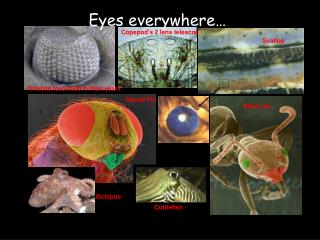
Eyes everywhere…. Copepod's 2 lens telescope. Scallop. Trilobite fossil 500 million years. House Fly. Black ant. Octopus. Cuttlefish. Modeling fly phototransduction: how quantitative can one get?. Limits of modeling?. Comparative systems biology?.

E N D
Eyes everywhere… Copepod's 2 lens telescope Scallop Trilobite fossil 500 million years House Fly Black ant Octopus Cuttlefish
Modeling fly phototransduction:how quantitative can one get?
Limits of modeling? Comparative systems biology? • vertebrate phototransduction (rods, cones) • insect phototransduction • olfaction, taste, etc…
Fly photo-transduction Outline: • About the phenomenon • Molecular mechanism • Phenomenological Model • Predictions and comparisons with • experiment.
Fly photoreceptor cell Microvillus hv Na+, Ca2+ Rhodopsin 50nm 1.5 mm
Single photon response in Drosophila: a Quantum Bump “All-or-none” response Low light Henderson and Hardie, J.Physiol. (2000) 524, 179 Dim flash
Comparison of a fly with a toad. Single photon response: Note different scales directions of current!! From Hardie and Raghu, Nature 413, (2001)
Linearity of macroscopic response hv Linear summation over microvillae
Average QB wave-form QB aligned at tmax Henderson and Hardie, J.Physiol. (2000) 524, 179 A miracle fit:
Latency distribution # of events Latency (ms) QB variability # events Peak current Jmax (pA)
Multi-photon response Macroscopic response = average QB Convolution with latency distribution QB waveform Latency distribution determines the average macroscopic response !!! Fluctuations control the mean !!!
Advantages of Drosophila photo-transduction as a model signaling system: • Input: Photons • Output: Changes in membrane potential • Single receptor cell preps • Drosophila genetics
Gabg * * * GDP Ga IP3 + DAG PLCb PKC Rh Rh DAG hv GTP GDP GTP Trp Na+, Ca++ Trp* Ca pump Response initiation High [Na+], [Ca++] PIP2 Low [Na+], [Ca++] DAG Kinase Cast: Rh = Rhodopsin; Gabg = G-protein PIP2 = phosphatidyl inositol-bi-phosphate DAG = diacyl glycerol PLCb = Phospholipase C -beta ; TRP = Transient Receptor Potential Channel
High [Ca++] Gabg GDP PIP2 IP3 + DAG PLCb PKC * * * Rh Ga DAG hv GTP Trp* GTP GDP Trp Na+, Ca++ Intermediate [Ca++] Positive Feedback Ca pump Intermediate [Ca] facilitates opening of Trp channels and accelerates Ca influx.
Gabg GDP PIP2 IP3 + DAG PLCb * * * Ga * * GTP Arr Trp* GTP GDP ?? Cam Negative feedback and inactivation High [Ca++] Rh* PKC Na+, Ca++ High [Ca++] Ca pump Cast: Ca++ acting directly and indirectly e.g. via PKC = Protein Kinase C and Cam = Calmodulin Arr = Arrestin (inactivates Rh* )
Comparison of early steps Vertebrate Drosophila 2nd messengers DAG cGMP From Hardie and Raghu, Nature 413, (2001)
…and another cartoon c. a. d b. From Hardie and Raghu, Nature 413, (2001)
InaD signaling complex InaD PDZ domain scaffold From Hardie and Raghu, Nature 413, (2001)
Speed and space: the issue of localization and confinement. Order of magnitude estimate of activation rates: PLC* ~ k [G] ~ 10mm2/s 100 / .3 mm2 > 1 ms-1 G* ~ ! Fast Enough ! Diffusion limit on reaction rate Protein (areal) density However if: ~ 1mm2/s 10 / .3 mm2 =.03ms-1 << 1 ms-1 ! Too Slow ! Possible role for InaD scaffold !
A naïve model low “Input” Ca2+ TRP channel ( G*, PLCb*, DAG) high
Kinetic equations: Activation stage ( G-protein; PLCb; DAG ): Input (Rh activity) QB “generator” stage ( Trp, Ca++ ): Positive and negative feedback # open channels Ca++ influx via Trp* Ca++ outflow/pump
Feedback Parameterization Parameterized by the “strength”ga(~ ratio at high/low [Ca]) Characteristic concentration KDa and Hill constant ma Note: this has assumed that feedback in instantaneous…
A=.2 Trp*/Trp .05 .03 A=.02 [Ca]/[Ca0] Null-clines and fixed points [Ca]=0 [TRP*]=0 null-cline
Problems with the simple model Experiment Model “High” fixed point • In response to a step of Rh* activity (e.g. in Arr mutant ) • QB current relaxes to zero • Ca dynamics is fast rather than slow no “overshoot” • Long latency is observed
Order of magnitude estimate of Ca fluxes [Ca]dark ~ .2mM 1 Ca ion / microvillus [Ca]peak ~ 200mM 1000 Ca ion / microvillus Note: m-villus volume ~ 5*10-12 ml Influx 104 Ca2+ / ms 30% of 10pA Hence, Ca is being pumped out very fast ~ 10 ms-1 [Ca] is in a quasi-equilibrium
Microvillus as a Ca compartment Ca++ 50nm 1-2 um Compare 10 ms-1 with diffusion rate across the microvillus: t -1 ~ Dca / d2 ~ 1mm2/ms / .0025 mm2 = 400 ms -1 But diffusion along the microvillus: is too slow compared to 10ms-1 t -1 ~ 1mm2/ms / 1 mm2 = 1 ms -1 Hence it is decoupled from the cell. Note: microvillae could not be > .3mm in diameter, i.e it is possible the diameter is set by diffusion limit
Slow negative feedback Assume negative feedback is mediated by a Ca-binding protein (e.g. Calmodulin??) Slow relaxation
A more ‘biochemically correct’ model: Cascade Feedback F+ F- Delayed Ca negative feedback
Stochastic effects Numbers of active molecules are small ! e.g. 1 Rh*, 1-10 G* & PLC*, 10-20 Trp* Chemical kinetics Reaction “shot” noise. Master equation Numerical simulation Gillespie, 1976, J. Comp. Phys. 22, 403-434 see also Bort,Kalos and Lebowitz, 1975, J. Comp. Phys. 17, 10-18
Stochastic simulation Event driven Monte-Carlo simulation a.k.a. Gillespie algorithm Gillespie, 1976, J. Comp. Phys. 22, 403-434 see also Bort,Kalos and Lebowitz, 1975, J. Comp. Phys. 17, 10-18 Numbers of molecules (of each flavor) #Xa(t) are updated #Xa(t) #Xa(t) +/- 1 at times ta,i distributed according to independent Poisson processes with transition rates Ga,+/- . Simulation picks the next “event” among all possible reactions. Note: simulation becomes very slow if some of the Reactions are much faster then others. Use a “hybrid” method.
The model is phenomenological… Many (most?) details are unknown: e.g. Trp activation may not be directly by DAG, but via its breakdown products; Molecular details of Ca-dependent feedback(s) are not known; etc, etc BUT there’s much to be explained on a qualitative and quantitative level…
Identifying “submodules” Cascade Key dynamical variables define “Submodules” Feedback F+ F- Delayed Ca negative feedback
Rephrased in a “Modular” form: the “ABC model” Activator – Buffer – Ca-channel Ca++ (PLCb*, Dag) “Input” Activator Channel (TRP) ( Rh*, G*) Ca++ B (Ca-dependent inhibition)
Quantum Bump generation (A,B) - “phase” plane High probability of TRP channel opening 180 TRP* 140 A 100 PLC* B*/10 60 A 20 0 200 400 600 B* “INTEGRATE & FIRE” process Threshold for QB generation
C 0 1 2 3 4 B What about null-cline analysis? Problems: • 3 variables A,B,C • Stochasticity • Discreteness Generalized “Stochastic Null-cline” “Ghost” fixed point
Can one calculate anything? E.g. estimate the threshold for QB generation: PLC* PLC* A-1 A A+1 Positive feedback kicks in once channels open Am Am f([Ca]) C = 0 1 2 Threshold A = AT such that Prob (AT -> AT +1) = Prob (C=0 -> C=1) NOTE: Better still to formulate as a “first passage” problem
Condition for QB generation Prob (C=1 C=2) > Prob (C=1 C=0) AT > AQB ([Ca]) Reliable QB generation AT Amax~ PLC* PLC* [Ca] * 4 3 AQB ([Ca]) 2 1 0 A [Ca] Bistable region/ Bimodal response
Quantum Bump theory versus reality Model Experiment Latency histogram Average QB profile
Fitting the data: QB wave-form There is a manifold of parameter values providing good fit for < QB > shape !! Trp*/Trptot Time (arbs)
So what ??? “With 4 parameters I can fit an elephant and with 5 it will wiggle its trunk.” E. Wigner
Non-trivial “architectural” constraints • Despite multiplicity of fits, certain constraints emerge: • Trp activation must be cooperative • Activator intermediate must be relatively stable: • “integrate and fire” regime. • Negative feedback must be delayed • Multiple feedback loops are needed • Etc, … Furthermore: Fitting certain relation between parameters: “phenotypic manifold” - the manifold in parameter space corresponding to the same quantitative phenotype.
Constraining the parameter regime… Help from the data on G-protein hypomorph flies: • # of G-proteins reduced by ~100 • QB “yield” down by factor of 103 • Increased latency (5-fold) • Fully non-linear QB with amplitude reduced about two-fold
G-protein hypomorph Model: Experiment: • Single G* and PLC* can evoke a QB !! • Reduced yield explained by PLC* deactivating • before A reaches the QB threshold • Relation between yield reduction and • increased latency. # PLC* ~ 5 for WT
What happens in response to continuous activation ? e.g. if Rh* fails to deactivate
Persistent Rh* activity Relaxation Oscillator (A,B*) phase plane 180 Trp* 140 A 100 B* 60 20 A 100 200 300 400 500 B* Unstable Fixed Point
QB trains: theory versus experiment Arrestin mutant (deficient in Rh* inactivation): Model: Qualitative but not quantitative agreement so far…