Direct Methods for Aibo Localization
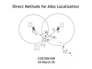
r 2 r 1 y x Direct Methods for Aibo Localization CSE398/498 04 March 05 Administration Plans for the remainder of the semester Localization Challenge Kicking Challenge Goalie Challenge Scrimmages Finish CMU Review Direct methods for robot localization

Direct Methods for Aibo Localization
E N D
Presentation Transcript
r2 r1 y x Direct Methods for Aibo Localization CSE398/498 04 March 05
Administration • Plans for the remainder of the semester • Localization Challenge • Kicking Challenge • Goalie Challenge • Scrimmages • Finish CMU Review • Direct methods for robot localization • Mid-semester feedback questionnaire
References • “CMPack-02: CMU’s Legged Robot Soccer Team,” M. Veloso et al • “Visual Sonar: Fast Obstacle Avoidance Using Monocular Vision,” S. Lenser and M. Veloso, IROS 2003, Las Vegas, USA
Visual Sonar • Based entirely upon color segmentation • The main idea: • There are only a handful of colors on the field • Each color can be associated with one or more objects • green -> field • orange -> ball • white -> robot or line • red or blue -> robot • cyan or yellow -> goal http://www-2.cs.cmu.edu/~coral-downloads/legged/papers/cmpack_2002_teamdesc.pdf
Visual Sonar (cont’d) • Based entirely upon color segmentation • The main idea: • Discretize the image by azimuth angle • Search in the image from low elevation angle to high for each azimuth angle • When you hit an interesting color (something not green), evaluate it • You can infer the distance to an object for a given azimuth angle from the elevation angle and the robot geometry http://www-2.cs.cmu.edu/~coral-downloads/legged/papers/cmpack_2002_teamdesc.pdf
Visual Sonar (cont’d) • By panning head you can generate a 180o+ range map of the field • Subtleties: • Identifying tape • Identifying other robots??? • Advantages over IRs • Video Link http://www-2.cs.cmu.edu/~coral-downloads/legged/papers/cmpack_2002_teamdesc.pdf
A Similar Approach… • Based entirely upon edge segmentation • The main idea: • All edges are obstacle • All obstacle must be sitting on the ground • Search in the image from low elevation angle to high for each bearing angle • When you hit an edge, you can infer the distance to an obstacle for a given bearing angle from the elevation angle
Why Does this Work? • Recall that edges correspond to large discontinuities in image intensity • While the carpet has significant texture, this pales in comparison with the white lines and green carpet (or white Aibos and green carpet)
Why Does this Work? (cont’d) • Let’s look at a lab example • OK, that did not work so great because we still have a lot of spurious edges from the carpet that are NOT obstacles • Q: How can I get rid of these? • A: Treat these edges as noise and filter them. • After applying a 2D gaussian smoothing filter to the image we obtain…
Position Updates • Position updates are obtained using the field markers and the goal edges • Both the bearing and the distance are estimated to each field marker. • To estimate the pose analytically, the robot needs to view 2 landmarks simultaneously • CMU uses a probabilistic approach that can merge individual measurement updates over time to estimate the pose of the Aibo • We will discuss this in more detail later in the course
+ The Main Idea… • Flashback 3 weeks ago • Let’s say instead of having 2 sensors/sensor model, we have a sensing and a motion model • We can combine estimate from our sensors and our motion over time to obtain a very good estimate of our position • One “slight” hiccup…
The Kidnapped Robot Problem • If you are going to use such probabilistic approaches you will need to account for this in your sensing/motion model
Summary • We reviewed much of the sensing & estimation techniques used by the recent CMU robocup teams • Complete reliance on the vision system – primarily color segmentation • Newer approaches also rely heavily on line segmentation – we may not get to this point • There is a lot of “science” in the process • There are a lot of heuristics in the process. There work well on the Aibo field, but not in a less constrained environment • Approaches are similar to what many other teams are using • Solutions are often not pretty - often the way things are done in the real world
References • A. Kelly, Introduction to Mobile Robots Course Notes, “Position Estimation 1-2” • A. Kelly, Introduction to Mobile Robots Course Notes, “Uncertainty 1-3”
Robot Localization • The first part of the robot motion planning problem was “Where am I” • Localization refers the ability of the robot to infer its pose (position AND orientation) in the environment from sensor information • We shall examine 2 localization paradigms • Direct (or reactive) • Filter base approaches
Direct (or Reactive) Localization • This technique takes the sensor information at each time step, and uses this to directly estimate the robot pose. • Requires an analytical solution from the sensor data • Memoryless • Pros: • Simple implementation • Recovers quickly from large sensor errors/outliers • Cons: • Requires precise sensor measurements to obtain an accurate pose • May require multiple sensors/measurements • Example: GPS
High Level Vision: Marker Detection • Marker detection will (probably) be your basis for robot localization as these serve as landmarks for pose estimation • Need to correctly associate pairs of segmented regions with the correct landmarks * www.robocup.org
Range-based Position Estimation r1 r2 • One range measurement is insufficient to estimate the robot pose estimate • We know it can be done with three (on the plane)? • Q: Can it be done with two? • A: Yes.
r1 r2 y x Range-based Position Estimation (cont’d) • We know the coordinates of the landmarks in our navigation frame (“field” frame) • If the robot can infer the distance to each landmark, we obtain • Expanding these and subtracting the first from the second, we get: which yields 1 equation and 2 unknowns. However, by choosing our coordinate frame appropriately, y2=y1
r1 r2 y x Range-based Position Estimation (cont’d) • So we get • From our first equation we have which leaves us 2 solutions for yr. • However by the field geometry we know that yr ≤ y1, from which we obtain
y x Range-based Position Estimation (cont’d) • So we get • From our first equation we have which leaves us 2 solutions for yr. • However by the field geometry we know that yr ≤ y1, from which we obtain r1 r2 ISSUE 1: The circle intersection may be degenerate if the range errors are significant or in the vicinity of the line [x2-x1, y2-y1]T
r1 r2 y x Range-based Position Estimation (cont’d) • So we get • From our first equation we have which leaves us 2 solutions for yr. • However by the field geometry we know that yr ≤ y1, from which we obtain ISSUE 2: Position error will be a function of the relative position of the dog with respect to the landmark
Error Propagation from Fusing Range Measurements (cont’d) • In order to estimate the Aibo position, it was necessary to combine 2 imperfect range measurements • These range errors propagate through non-linear equations to evolve into position errors • Let’s characterize how these range errors map into position errors • First a bit of mathematical review…
Error Propagation from Fusing Range Measurements (cont’d) • Recall the Taylor Series is a series expansion of a function f(x) about a point a • Let y represent some state value we are trying to estimate, x is the sensor measurement, and f is a function that maps sensor measurements to state estimates • Now let’s say that the true sensor measurement x is corrupted by some additive noise dx. The resulting Taylor series becomes • Subtracting the two and keeping only the first order terms yields
Error Propagation from Fusing Range Measurements (cont’d) • For multivariate functions, the approximation becomes where the nxm matrix J is the Jacobian matrix or the matrix form of the total differential written as: • The determinant of J provides the ratio of n-dimensional volumes in y and x. In other words, |J| represents how much errors in x are amplified when mapped to errors in y
Error Propagation from Fusing Range Measurements (cont’d) • Let’s look at our 2D example to see why this is the case • We would like to know how changes in the two ranges r1 and r2 affect our position estimates. The Jacobian for this can be written as • The determinant of this is simply • This is the definition of the vector (or cross) product
Error Propagation from Fusing Range Measurements (cont’d) v1 v2 • Flashback to 9th grade… • Recall from the definition of the vector product that the magnitude of the resulting vector is • Which is equivalent to the area of the parallelogram formed from the 2 vectors • This is our “error” or uncertainty volume
r1 r2 y x Error Propagation from Fusing Range Measurements (cont’d) • For our example, this means that we can estimate the effects of robot/landmark geometry on position errors by merely calculating the determinant of the J • This is known as the position (or geometric) dilution of precision (PDOP/GDOP) • The effects of PDOP are well studied with respect to GPS systems • Let’s calculate PDOP for our own 2D GPS system. What is the relationship between range errors and position errors?
Position Dilution of Precision (PDOP) for 2 Range Sensors The take-home message here is to be careful using range estimates when the vergence angle to the landmarks is small • The blue robot is the true poistion. • The red robot shows the position • estimated using range measurements • corrupted with random Gaussian noise • having a standard deviation equal to • 5% of the true range
Error Propagation from Fusing Range Measurements (cont’d) Bad Good QUESTION: Why aren’t the uncertainty regions parallelograms? Bad
y x Inferring Orientation • Using range measurements, we can infer the position of the robot without knowledge of its orientation θ • With its position known, we can use this to infer θ • In the camera frame C, the bearings to the landmarks are measured directly as • In the navigation frame N, the bearing angles to the landmarks are • So, the robot orientation is merely NOTE: Estimating θ this way compounds the position error and the bearing error. If you have redundant measurements, use them.
x y Bearings-based Position Estimation • There will most likely be less uncertainty in bearing measurements than range measurements (particularly at longer ranges) • Q: Can we directly estimate our position with only two bearing measurements? • A: No.
Bearings-based Position Estimation • The points (x1,y1), (x2,y2), (xr,yr) define a circle where the former 2 points define a chord (dashed line) • The robot could be located anywhere on the circle’s lower arc and the inscribed angle subtended by the landmarks would still be |α2- α1| • The orientation of the dog is also free, so you cannot rely upon the absolute bearing measurements. • A third measurement (range or bearing is required to estimate position) NOTE: There are many other techniques/constraints you can use to improve the direct position estimate. These are left to the reader as an exercise.
r1 r2 Range-based Position Estimation Revisited • We saw that even small errors in range measurements could result in large position errors • If the noise is zero-mean Gaussian, then averaging range measurements should have the effect of “smoothing” (or canceling) out these errors • Let’s relook our simulation, but use as our position estimate the average of our 3 latest position estimates. In other words…
Position Estimation Performance forDirect and 3-element Average Estimates Direct Estimate Mean Filter • The blue robot is the true poistion. • The red robot shows the position • estimated using range measurements • corrupted with random Gaussian noise • having a standard deviation equal to • 5% of the true range
Position Error Comparison Position Estimates Errors from 3 element Mean Filter Direct Position Estimate Errors (unfiltered) • Averaging is perhaps the simplest technique for filtering estimates over time • We will discuss this in much greater detail after the break