Download
1 / 26
260 likes | 375 Vues
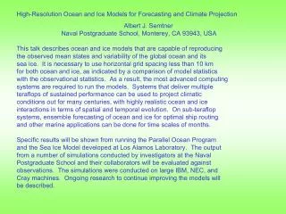
High-Resolution Ocean and Ice Models for Forecasting and Climate Projection

E N D
High-Resolution Ocean and Ice Models for Forecasting and Climate Projection Albert J. Semtner Naval Postgraduate School, Monterey, CA 93943, USAThis talk describes ocean and ice models that are capable of reproducingthe observed mean states and variability of the global ocean and itssea ice. It is necessary to use horizontal grid spacing less than 10 kmfor both ocean and ice, as indicated by a comparison of model statisticswith the observational statistics. As a result, the most advanced computingsystems are required to run the models. Systems that deliver multipleteraflops of sustained performance can be used to project climaticconditions out for many centuries, with highly realistic ocean and iceinteractions in terms of spatial and temporal evolution. On sub-teraflopsystems, ensemble forecasting of ocean and ice for optimal ship routingand other marine applications can be done for time scales of months.Specific results will be shown from running the Parallel Ocean Programand the Sea Ice Model developed at Los Alamos Laboratory. The outputfrom a number of simulations conducted by investigators at the NavalPostgraduate School and their collaborators will be evaluated againstobservations. The simulations were conducted on large IBM, NEC, andCray machines. Ongoing research to continue improving the models willbe described.
Navy Prediction Vision • A high-resolution global coupled air/ocean/ice prediction system (via NOGAPS - Navy Operational Global Atmospheric Prediction System, plus suitable ocean and ice models not yet finalized) • Very-high resolution regional coupled models nested into the global system at strategic locations .(via COAMPS - Coupled Ocean Atmosphere Mesoscale Prediction System) • A coupled Pan-Arctic ice-ocean model that provides operational forecasts of sea ice and ocean conditions. (via PIPS - Polar Ice Prediction System)
Parallel Ocean Program (POP) • Primitive equation z-level ocean model with active thermodynamics • A modern descendent of the “GFDL Bryan-Cox ocean model”, developed and supported by a group at Los Alamos National Laboratory • 3-D “baroclinic” variables are explicitly timestepped; however, 2-D equations for the vertically averaged “barotropic” flow and free surface elevation are implicitly treated (leading to global sums in solving for the latter). • Fortran90 • Designed to run on multi-processor machines using domain decomposition in latitude and longitude • MPI for inter-processor communications on distributed memory machines and SHMEM on shared memory machines
0.1 40-level global POP SST SSH McClean (NPS) and Maltrud (LANL)
Grid size for this study Grid size of an earlier global simulation by Maltrud, Smith, Semtner, and Malone,1998) following
High resolution is needed for proper jet separation
Principal standard deviation ellipses (cm/sec) from 2x2 binned North Atlantic surface drifter velocity data (green), 0.28(blue), and 0.1 POP (red) velocity output for 1993-1997 High resolution is needed for correct mean path of Gulf Stream.
Courtesy, Robin Tokmakian Times series of SSHA (cm) from NA 0.1 POP (red) and tide gauges for 1993-1998.
Fully Global Displaced North Pole Grid Pole is rotated into Hudson Bay to avoid polar singularity. In the northern hemisphere mid-latitudes the highest horizontal resolution is off east and west coasts of the U.S Average grid spacing over all ocean points is ~6.5 km.
Performance Statistics One year of simulation requires 8 DAYS on 500 IBM SP3 processors at DOD’s NAVO site (McClean and Maltrud). One year of simulation requires 8 HOURS on 960 NEC SX6 processors of the Earth Simulator (F. Bryan and CRIEPI collaborators)
Near Surface Speed May have to resolve the complex transfers of heat across the Circumpolar Current toward sea ice and ice shelves
Sea Surface Height May need to resolve eddy transport of heat northward in South Atlantic part of the global “Conveyor Belt”
Ongoing POP Improvements(underway at LANL) • More scalable barotropic solver • Hybrid OpenMP/MPI with better cache performance • Hybrid vertical coordinate • Partial bottom cells • Better subgrid closure schemes • Bottom boundary layer Parallel optimization Numerical accuracy Physics
Polar Ice Prediction System (PIP3.0) W. Maslowski et al. • Ocean model: POP (1280x720x45) has ~9 km near- constant grid spacing over the pan-Arctic region • Finite-difference sea-ice model equations for momentum, compactness, and thickness (same grid) • Viscous-plastic sea-ice rheology and simple thermodynamic heat transfer through ice • Developed and integrated as a DOD “grand challenge” project on the Cray T3E at the Arctic Region Supercomputing Center
LABRADOR SEA EDDY KINETIC ENERGY(cm2/s2) 18 KM VS 9 KM, August 1980 Snapshot 0-43 m (levels 1-2) 0-45 m (levels 1-7) • Order of magnitude increase in EKE from 18 km to 9 km • 9 km values approaching observed ones (not shown) • Eddy activity preconditions deep convection here and in the Greenland/Norwegian Sea => high resolution needed
A snapshot of (a) ice area and drift, (b) divergence, (c) shear, and (d) vorticity- Spinup 08/01/79 (b) (a) (d) (c) Inclusion of leads, polynyas, and ridges requires high resolution.
Los Alamos Sea Ice Model:CICEHunke, Bitz, Lipscomb • Multicategory ice thickness, presently 4 ice layers plus snow • Elastic-Viscous-Plastic dynamics (for better parallelism) • 2-D re-mapping scheme for improved horizontal ice transport • Ridging parameterization for updating the thickness distribution
Multi-category Sea Ice Concentrations (%) – September 1, 1982 (Maslowski and Lipscomb) Total (%) and Drft (m/s) Category I (0-0.45 m) Category II (0.45-1.2m) Category III (1.2-2.2 m) Category IV (2.2-4.5 m) Category V (4.5-9.0 m) Allows proper treatment of the non-linear dependence of both dynamics and thermodynamics on ice thickness distribution.
Conclusions High-resolution models of the Global Ocean, the Arctic Ocean and sea ice: - correctly represent critical aspects of the mean features and their eddy dynamics, many of which may not be representable in coarse-grid models - have the potential to make predictions on short to long time scales when used with atmospheric models - require large blocks of supercomputer time, especially for extended integrations