Rethinking Routing in Dynamic Networks: Beyond Graphs and Static Models
250 likes | 367 Vues
In this presentation, Dmitri Krioukov explores the limitations of traditional graph-based routing in dynamic, large-scale networks. He emphasizes the need to reassess fundamental assumptions about information transmission, addressing challenges posed by self-organizing networks and the inherent dynamic nature of routing. By introducing novel concepts such as non-hierarchical routing and compact routing functions, the talk delves into the potential for new paradigm shifts in network design. Krioukov discusses practical implementations and examples, advocating for adaptive approaches to contemporary networking problems.

Rethinking Routing in Dynamic Networks: Beyond Graphs and Static Models
E N D
Presentation Transcript
Flat Routing on Curved Spaces Dmitri Krioukov(CAIDA/UCSD) dima@caida.org Berkeley April 19th, 2006
Clean slate:reassess fundamental assumptions • Information transmission • between nodes • in networks that are • large-scale and growing • dynamic and more dynamic • self-* and more *
Dynamics • graphs are no longer good network abstractions • graphs are static, networks are dynamic • routing ‘without graphs’ (paradigm shifts) • reinforcement learning… • operations (e.g., for DTNs)… • multicommodity flow problem • physical routing • too hard to shift paradigms and live without graphs • NP-hardness everywhere • approximations are slow • media required for physical routing does not seem to exist • let’s not shift paradigms now and check if we’ve done everything we can about graphs
Self-* • many examples of large-scale self-grown/organized networks • all of them have • power-laws • with γ ~ 2.1 • small-world • small average distances and diameters • consequence of power-laws • strong clustering • not a consequence of power-laws • e.g.: AS-level topo and topo of metabolic reactions are just the same
hierarchical location address name-dependent non-hierarchical ID name name-independent Routing (with graphs)
good when network is static has a ‘nice structure’ trees are best (that’s why we use word hierarchical): you can route along shortest paths with logarithmic routing tables with constant lookup times bad when network is dynamic have to rename nodes! ‘unstructured’ Hierarchy/name-dependence is:
Hierarchy/name-dependence • is recognized as a scalability problem both in • theoretical community, and • networking community
Non-hierarchical/flat routing ideas • DHTs • name-independent compact routing
DHT idea • problem formulation • given • some metric space M (that is, ‘underlay’) • find • map: M→ E s.t. routing in E is ‘easy’ (e.g., scales infinitely) • standard choice of E is an Euclidean space, since routing in Euclidean spaces is no problem • existence of angles gives a sense of direction (‘just go `there`’) • routing table sizes are constant (don’t depend on the network size) • greedy routing is shortest path routing, • but: in E, not in M!
Compact routing (CR) • problem formulation • given • graph G (so is its metric space!) • find • map (routing function): (s, t) → ps (where s is a source (or current node), t is a target, ps is a port at s on the path to t), s.t. routing table size (memory space) and path lengths (stretch) are nicely balanced • name-dependent (ND) • routing can rename nodes as needed (e.g., injecting some topological information into node names) in order to make routing easier • name-independent (NI) • nodes names are also given (e.g., from a flat space) and cannot be changed
DHTs vs. NICR (main point) NICR does not require underlay it works on a given topology
CR ideas n n = n (n1/k)k = n
NI ideas n n = n
NDCR example(stretch: 3, space: O(n)) • neighborhoods (clusters): my neighborhood is a set of nodes closer to me than to their closest landmarks • landmark set (LS) construction: iterations of random selections of nodes to guarantee the right balance between the neighborhood size (O(n)) and LS size (O(n))! • routing table: shortest paths to the nodes in the neighborhood and landmarks • naming: original node ID, its closest landmark ID, the ID of the closest landmark’s port lying on the shortest path from the landmark to the node • forwarding at node v to destination d: • if v = d, done • if d is in the routing table (neighbor or landmark), use it to route along the shortest path • if v is d’s landmark, the outgoing port is in the destination address in the packet, use it to route along the shortest path • default: d’s landmark in the destination address in the packet and the route to this landmark is in the routing table, use it
NICR example (for metric spaces)(stretch: 3, space: O(n)) • neighborhoods (balls): my neighborhood is a set of O(n)nodes closest to me • coloring: color every node by one of O(n) colors (O(n) color-sets containing O(n) nodes each), s.t. every node’s neighborhood contains at least one representative of every color (all colors are ‘everywhere dense’ in the metric space) • hashing names to colors: just use first log(n) bits of some hash function values (it’s ok w.h.p.) • routing table: nodes in the neighborhood and nodes of the same color • forwarding at node v to destination d: • if v = d, done • if d is in the routing table (neighbor or v’s color), use it to route along the shortest path • default: forward to v’s closest neighbor of d’s color • has been implemented and deployed (overlay ‘tulip’ on planetlab)
NICR example (for graphs)(stretch: 3, space: O(n)) • LS set: all nodes l of one selected color • NDCR on trees: every node resides in O(n) of such trees T: • routing table of v: • shortest-path links to neighbors • T(l,v) for all landmarks l (i.e., the routing table produced for v by NDCR on the shortest-path tree rooted at l) • T(x,v) for all neighbors x • for all nodes u of v’s color, either (whatever corresponds to a shorter path): • info for path in T(lu) (v→T(lu)→u), or • info for path via w, where w is s.t.: 1) v is a w’s neighbor, and 2) w’s and u’s neighborhoods are one hop away from each other (v→w→ x → y →u, where v,x are w’s neighbors and y is u’s neighbor) • forwarding at node v to destination d: • if v = d, done • if d is in the routing table (neighbor or landmark or v’s color), use it • default: forward to v’s closest neighbor of d’s color
NICR ideas • use NDCR underneath • no surprise since still need to locate the target, quite a fundamental ‘problem’ • use the graph’s metric structure to encode how the information on mapping of given (flat) names to NDCR addresses is distributed among nodes in a balanced n n manner • examples of other NI tricks (from other schemes):split n names into n blocks containing n names each, and agree that: • i’th farthest node from me keeps NI2ND tables for i’th block, or • do BFS rooted at me, node with BFS number i keeps NI2ND tables for i’th block • etc.
Generic/universal schemes • lower bounds • shortest path (s = 1) (n) • 1 s < 3 (n) • 3 s < 5 (n) • upper bounds • ND, s = 3, O(n2/3), Cowen, SODA’99 • ND, s = 3, O(n), Thorup&Zwick, SPAA’01 • NI, s = 5, O(n), Arias et al., SPAA’03 • NI, s = 3, O(n), Abraham et al., SPAA’04
Direction change:from generic to specific • average case is much better than the worst case(as always with complexity ) • realistic case is even better(as often with complexity )
Design specifically for realistic (scale-free) topologies • Brady&Cowen, ALENEX’06 • extract d-core (nodes at maximum distance d from the highest degree node) to achieve ‘right’ balance between d and e, the number of edges to remove from the fringe (graph \ core) to make it forest • additive stretch = d, space O(e) • Carmi, Cohen&Havlin, in progress • find H highest degree nodes (hubs) • name nodes by the paths to their closest hubs • store routes to all hubs and 1-hop neighbors • route either to the neighbor, or down the path if i’m a part of the name, or up to the destination’s hub in the name • average stretch is small, space is O(H + kmax)
Scale-free networks are theoretically challenging • not so much of mathematically rigorous results • too diverse communities involved (networking, CS theory, physics, math, statistics) • efforts in different directions, attempts to sync up (e.g., last year: Aldous’s workshop at MSRI; this year: CAIDA’s WIT, Barabasi’s, Bollobas’s workshops, etc.)
CS theory decides not to wait • routing on graphs • with bounded doubling dimension • α is the graph’s doubling dimension if every ball of radius 2r can be covered by at most αballs of radius r • unfortunately, distance distributions in realistic networks approach δ-functions in the large network limit, α is infinite in such networks • excluding a fixed minor • minor is a graph that can be obtained from a given graph by vertex/edge deletions and/or edge contractions • Robertson&Seymor’s deep structure theorem: for any class of graphs closed under minor-taking, there is a finite obstruction set of graphs that cannot be obtained as minors (e.g., trees exclude K3, planar graphs exclude K5 and K3,3) • connection to treewidth: for every planar H(V,E), there is constant c, s.t. for every G, if H is not G’s minor, then G’s treewidth is at most c (c can be large though, e.g., 204|V|+8|E|5) • treewidth of graph G: • is the minimal width of G’s treewidth decomposition T (the minimum is taken over all possible T’s) • treewidth decomposition T is a tree whose nodes are called bags, they are subsets of G’s nodes, s.t.: • the union of all bag is all G’s nodes • every pair of adjacent nodes in G resides in at least one bag • for any G’s node, the set of bags containing it forms a subtree in T • width of T is its maximum bag size minus 1 • treewidth measures the accuracy of approximation of G’s topology by a tree; recall that routing on trees is easy! • searching on graphs
Graph searching • Milgram’s expreiments, 1967 • Kleinberg model, 2000 • d-dimensional grid augmented with long-range links with harmonic distribution (ρ(x,y)-α) • routing is greedy in the underlying grid, excluding long-range links • phase transition (polynomial-to-polylogarithmic number of routing hops) at the ‘right’ form of the long-range distribution (α = d) • Fraigniaud model, 2005 • a graph with bounded treewidth or strong clustering(!) augmented with long-range links to centroids of subtrees of the graph’s treewidth decomposition • Kleinberg’s review and open problems, 2006
Graph searching hype • attempts to formalize efficient routing without global view (no M or G is given!!!) • possesses infinite scalability (assuming neighborhoods do not explode) • supports highly dynamic networks (assuming there is a relatively static meta-topology) • naturally supports any kind of (flat) topologies (assuming they can be decomposed into local and global parts that are ‘nice’) • is closest to being analytically solvable in the case with realistic networks • bottom line: searching is what you mostly do on the Internet today anyway, so why all the nodes should keep routing state about all the destinations all the time?
Main points about routing • topology matters (and even more so, according to the recent progress) • knowing only my neighborhood, the microscopic structure of the network, can i efficiently route globally, through its macroscopic structure? • some existing tools helpful for initial tests trying to answer the question: • Chung’s hybrid model • minors, treewidth • dK-series • connection to the network evolution via inverting the problem: maybe navigation easiness is one of the forces behind the evolution of large-scale self-* networks (Clauset&Moore) • things to try (further) in the nearer future • NICR • graph searching