Covariance Forecasting for Portfolio Optimization at R/Finance Chicago May 2013
240 likes | 338 Vues
Explore the estimation and forecasting of covariance for portfolio optimization using factors such as APT, CAPM, PCA, and more. Learn about factor analysis, principal components analysis, and the application of Bayesian shrinkage. Discover how to handle missing data, test for breakdowns, and conduct variance tests across different estimation universes.

Covariance Forecasting for Portfolio Optimization at R/Finance Chicago May 2013
E N D
Presentation Transcript
Covariance forecasting for portfolio optimisation R/Finance Chicago May 2013
Package aa: repeatable backtest simulation for equities Package aa Three inputs (universe, library, parameters) all logged in the database The user’s ‘alpha library’ operates on zoo/xts objects from SQL database Estimation and forecasting of covariance is central RGtk2 RDCOMClient MySQL tables via RODBC
CAPM, the APT, PCA and all that • Arbitrage Pricing Theory (APT) • If factor 1 is ‘the market’, CAPM nests into APT • factors 2:k remain to be specified • Identifying the factors • Regression: cross-sectional loadings known a priori • Size • Value etc … • Industry (directional) • Regression: timeseries scores known a priori • Market (directional) • Bond yield changes • Oil price changes • Surprises in general • PCA-type: scores are ‘portfolio’ returns • Exists a choice: ‘the answer in finite samples is not clear’ • Factor Analysis • Principal Components Analysis APT and PCA returns loadings scores specific returns APT (blue) CAPM (red) PCA (blue) CAPM (red) These Google trends graphs are for entertainment only!
Principal Components Analysis • PCA as ‘dimension reduction’ • eigenvalues are descending in magnitude • covariance can be summarised with the first k • precisely fits the bill for APT if stated as follows: • Remove off-diagonals for specific returns PCA Covariance Eigenvectors Eigenvalues Covariance illustration Example: 67 utilities 230 weeks 20 factors eigenvectors are orthonormal loadings scores (unit variance) specific returns
Tweaks • Part 1 : see package BurStFin • Model correlation, not variance • Handling missing data • Model ‘individuals’ (stocks) with complete data • ‘Regress in’ incomplete stocks, factors 1:k’ • Assign average loadings for lower-ranked factors • Iterate the process (repeat, starting from S*) • Part 2 : more niceties • Optimise the ‘factor portfolios’ • We had • Satisfies orthonormality but does not minimise specific risk • Use package quadprog for constrained optimisation • Apply Bayesian shrinkage • prior: , stronger for low eigenvalues • Missing data in cross-section • Frequent occurrence in global data • Substitute NA with 0, compute systematic returns, iterate • Inverse VIX scaling to make vol stationary • VIX is forward-looking option vol and a better forecast • Some smoothing is required, though PCA tweaks
Testing for breakdown: lag notation • Rolling estimates • We update models regularly to reflect changes • Further information can be extracted from them • Applied to the factor model estimate • Example: • Analyse all return(t) through a single estimate T* • Analyse single return(t*) through all estimates (T) • Take constant-lag (t*) panels • Negative lags are not feasible, they are in-sample • Zero lag is usual, means ‘using the latest estimate’ • Positive lags are feasible, mean ‘using older estimates’ • Application: consider the fit Lag notation Notation for rolling estimates lag return date model estimation date R2(t)
Testing for breakdown: regress returns on components • An augmented factor regression • kth factor: the ‘marginal’ explanatory power • deviation: cd<0 implies mean-reversion • quadratic: option-like payoff • #Testing the null • res <- summary(m1 <- lm(returns ~ Rm+ Rs+ Rl+ Rd+ Rq-1)) • linearHypothesis(m1,c(0,0,0,1,1))["Pr(>F)"] • linearHypothesis(m1,diag(5),c(1,1,1,0,0))["Pr(>F)"] Regression equation Define components of systematic return: etc market (factor 1) systematic (factors 2:k-1) kth factor deviation from mean quadratic Note: coefficients can be adjusted for ‘errors in the variables’ 0<cq for +ve gamma
Results from testing the model • Coefficients • Market and systematic components have coefficients close to 1 at lag 0 • Deviation shows • In-sample, less shrinkage for better fit (as expected) • Out of sample, more shrinkage for better fit (about -0.07 more, on top of -0.3 applied) • Evidence of mean-reversion as the coefficient decreases for greater lags • Quadratic term is pure noise Regression test results
Results from testing the model • Return variance/forecast variance • In general the lag-zero normalised variance is very close to 1 • Some evidence of slight under-forecasting of systematic components • (The trend upwards out-of-sample is period-specific, has no significance) Variance test results
Testing for breakdown: without adjustments • Without shrinkage or VIX • shows • Higher in-sample fit (0.68 vs 0.65) • Lower out-out-of-sample fit (0.46 vs 0.48) • underprediction is greater (1.49 vs 1.18) • These differences fit with expectations VIX and shrinkage
Testing across estimation universes • Results up to this point are averages across 7 global sectors • Here examine impact of sector size on the results • Report level of metric at and change from • R2 is lower for larger universes, where k/n is lower • No evidence of greater out-of-sample breakdown for larger universes Performance across universes
Universe selection • Requirements • No survivorship bias • Stable identifiers • Stationary screening criteria • A possible solution • Historical index constituents, screened • Issues with criteria, licencing • A specific solution • Bloomberg bworld = bworldus+bworldeu+bworldpr • Identifier ‘unique identifier’ or ‘open symbology’ • Screen on • Exchange, geographical, sector classification • Weight – maintains a fairly stationary universe composition • Liquidity • Alpha data coverage • Impact of eliminating biases • ‘distress’ type performance is sensitive • Turnover is higher Universe selection Realistic ex-ante Universe Date Date “Screened current constituents” Universe
Application 1: forecast-free portfolio construction • The ‘proxy basket’ • A small portfolio of closely matched stocks • Tracks the target stock with minimum variance • It is a constrained, optimal version of • Optional constraints • No shorting • Weights sum to unity • Uses • Hedging • Alpha-generation: mean-reversion and statarb • Application to valuation using yield-like variables • the basket is a risk-matched benchmark in the same industry • It is the single best ‘comp’ for valuation • Regression tests: on return or yield • require(quadprog) • x <- diag(n) • solve.QP(Dmat=ce,dvec=0,Amat=cbind(x[,i],x[,-i]), • bvec=c(1,rep(0,n)),meq=1) Proxy Basket Minimise: Subject to: Example: Gas Utilities, 2012-10
Application 2: market-neutral tilt portfolio • unconstrained solution defines • Forecast options • centred ranks: uniform distribution • ‘normalise’ using inverse cdf • Constraint options • Factor-1 neutral within sector/region • Factor 2:k neutral • Position size • Leverage options • Gross exposure () • Volatility • library(quadprog) • sol <- uniroot(f = tgtqp, interval = c(5, 0.05) * • objfun(w = solve(Dmat, dvec), Dmat = Dmat)/tgt, • Dmat= Dmat, dvec = dvec, constr = constr, • tgt= tgt, tol = 0.1, objfun = objfun)#(schematic) Market-neutral tilt tar Solve for Subject to: Equal forecasts Example: Utilities, 2011-10
Attribution • For a single period • Variance and return have the same components • Market (factor 1) • Systematic (factors 2:k) • Residual • Drilldown into category trees • Geographical tree (region, country, state) • Industrial classification tree (GICS, ICB, BICS) • Long, short subportfolios • Option to apply different trees on the two axes • Multi-period treatment of returns • ‘Simple’ with no compounding, or… • ‘Smoothing’ scheme, redistributing interactions • Contrast with Brinson/Fachler and extensions • No benchmark (cash benchmark) • Consequently no selection/allocation/interaction • Currency easy: • local returns vs local cash (hedged) • $ returns vs $ cash (unhedged) • Leverage easy: premia are self-financing Attribution Cash benchmark Brinson/Fachler
Mean-variance optimisation criticisms • Markowitz optimisation • Ignores sampling errors in the covariance matrix • Solves a mis-specified problem • Portfolio weights • Sensitive to sampling errors in covariance • Do not follow intuition • Are distant from true optimality • Utility and Sharpe Ratio • Variance is underestimated • Expected return is overestimated • ‘Solutions’ have been proposed • But how serious is the problem? • Might the answer depend on the risk model type? Optimisation The trivial read-across from Utility(w) -> Sharpe(w)
Optimisation: a monte-carlo test (1) • Using ‘vanilla’ PCA without shrinkage • From an estimated covariance matrix • Generate synthetic data • Re-estimate covariance from this • Draw expected return from a uniform distribution • Optimise • subject to industry group neutrality constraint • Adjusting risk-aversion to target volatility • Repeat for seven global equity sectors • Results • optimum and optimised weights correlate highly • True vol is 1.16x expected vol from the estimate • Expected return is 1.09x the true optimum Optimisation monte-carlo
Optimisation: a monte-carlo test (2) • Apply Bayesian shrinkage • Prior: , stronger for low eigenvalues • Prior weight is 0.3 for factor 1 loading • Underestimate of volatility is reduced • ; 11 • Conclude • Underestimation of volatility has been exaggerated • Higher return partially compensates • Optimisation is not ‘eating’ alpha or IR in this case Optimisation monte-carlo
Optimisation as a projection • An observation • Recall that for unconstrained optimisation • Or in recipe form: • Project E[R] onto eigenvectors by dotproduct • Divide by eigenvalues (!) • Scale eigenvectors accordingly and sum • Step 2 is the error-maximisation property • It relates to the condition number of the matrix • The correction has reduced this • Shrinkage reduces it further • Modified PCA reduces error amplification • Industry-level neutrality constraints • Reduce systematic risk • Condition the solution, largely driven by Optimisation as projection
A live application in real time: global equity market neutral • A contrarian low-frequency strategy run in real time as a ‘paper portfolio’ performed in-line with backtest • But too low vol: 8% for 8x leverage and net long, not $-neutral so not ‘market neutral’ despite beta=0 • Moral: be careful what your client asks for (diversification, hedging) - you might get it and still not like it Live Application • source: Bloomberg PORT Sharpe Ratio 2.91 Return/trade 0.72% Return/gross 3.30% Volatility/gross 1.14% Holding period 23 weeks Net/gross 6.3% source: internal
Application: the open source talent contest • There exists a severe barrier to entry in the capital management industry • Backtests have no credibility due to deliberate or unwitting exercise of hindsight options • Paper portfolios are a waste of time – trade at the touch, and one can run many • Move to a clear and transparent process with detailed reporting • Anonymous enrolment into accredited paper portfolios, executed at VWAP • Detailed drill-down reporting on positions, risk, liquidity , performance • Capital introduction / seeding from early investors Cap intro
Not just another backtest • We have seen • A framework for rigorous testing of an equity covariance model • Applications in backtest simulation of equity market neutral strategies • The latent demand for an open source equity risk and backtest system • The market for trading talent is highly imperfect due to secrecy • This is the missing mechanism for matching talent with capital whilst respecting IP • A bias-free backtest+ paper portfolio executed at VWAP can form the reference point • Traction at last for the backtest? Review Talent
Process: review and timings Process RDCOMClient MySQL tables via RODBC RGtk2
Attribution of performance, risk, position, directional vol • Attributions shown are derived by lagging position with respect to returns, similar to earlier lag of covariance • Shows that the strategy is contrarian, market neutral, residual risk, and symmetrical across long and short • The three shown are a subset of approximately 300 tabulations warehoused for rapid browsing Attributing performance Sector contribution Risk component contribution Cumulative performance (%) Long / Short contribution Lag (weeks) Live running 1-year period, all sectors average, bworld US + EU screened