Covariance Estimation For Markowitz Portfolio Optimization
Covariance Estimation For Markowitz Portfolio Optimization. Ka Ki Ng Nathan Mullen Priyanka Agarwal Dzung Du Rezwanuzzaman Chowdhury. Portfolio Selection Problem. Consider N stocks whose returns are distributed with mean μ and covariance matrix Σ


Covariance Estimation For Markowitz Portfolio Optimization
E N D
Presentation Transcript
Covariance Estimation For Markowitz Portfolio Optimization Ka Ki Ng Nathan Mullen PriyankaAgarwal Dzung Du RezwanuzzamanChowdhury
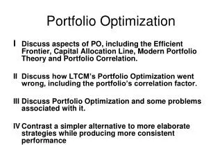
Portfolio Selection Problem • Consider N stocks whose returns are distributed with mean μ and covariance matrix Σ • Markowitz defines the portfolio selection problem as: where q is the required expected return • Solve it using Lagrange multipliers, the solution is:
Portfolio Selection Problem • Input: expected stocks returns and covariance matrix of the stock returns • Output: the efficient frontier (i.e. the set of portfolios with expected return greater than any other with the same or lesser risk, and lesser risk than any other with the same or greater return) • Global minimum variance portfolio (GMVP) doesn’t require the estimation of the expected stock returns
Portfolio Selection Problem • The problem is reduced to: • The solution is:
Covariance Matrix Estimators • Sample covariance matrix estimator: • Covariance matrix estimator implied by Sharpe’s single-index model: where s002 is the sample variance of the market returns, b is the vector of the slope estimates, and D is the diagonal matrix containing residual variance estimates • Ledoit and Wolf’s shrinkage (of S towards F) estimator: (weighted average of the single-index model and the sample matrix)
Data and Period of Study • Ledoit and Wolf’s paper • Use NYSE and AMEX stocks from August 1962 to July 1995 • For each year t from 1972 to 1994 • In-sample period: August of year t-10 to July of year t for estimation • Out-of-sample period: August of year t to July of year t+1 • Consider those with • valid CRSP returns for the last 120 months and future 12 months (Disatnikand Benninga's paper) • valid Standard Industrial Classification (SIC) codes • The resulting number of stocks used for constructing the GMVP varies across the years
Experiments • Used the estimated covariance matrices to compute the portfolio weights • Compute the returns of the portfolios for the out-of-sample period • Record the monthly returns for each portfolio • Compute the variances of the monthly returns for each portfolio over the 23-year period
Risk of Minimum Variance Portfolio Notes: Unconstrained refers to global minimum variance portfolio Standard deviation is annualized through multiplication by and expressed in percents
Optimal Shrinkage Intensity Estimate • This intensity is α from Ledoit and Wolf’s shrinkage estimator: (weighted average of the single-index model and the sample matrix) • They all have values ≈ 0.8, that means there is four times as much estimation error in the sample covariance matrix as there is bias in the single index model