Exploratory Factor Analysis
Exploratory Factor Analysis. Common factor analysis. This is what people generally mean when they say "factor analysis." This family of techniques uses an estimate of common variance among the original variables to generate the factor solution


Exploratory Factor Analysis
E N D
Presentation Transcript
Common factor analysis • This is what people generally mean when they say "factor analysis." • This family of techniques uses an estimate of common variance among the original variables to generate the factor solution • It is based on the fundamental assumption that some underlying factors, which are smaller in number than the observed variables, are responsible for the covariation among them
Factor Analysis • There are four basic steps: • data collection and generation of the correlation matrix • extraction of initial factor solution • rotation and interpretation (also validation) • construction of scales or factor scores to use in further analyses • A good factor: • Makes sense • Will be easy to interpret • Possesses simple structure • Items have low cross-loadings
Factor Analysis • Factor analysis can be seen as a family of techniques, of which both PCA and EFA are members* • Factor analysis is a statistical approach that can be used to analyze interrelationships among a large number of variables and to explain these variables in terms of their common underlying dimensions (factors) • It involves finding a way of condensing the information contained in a number of original variables into a smaller set of dimensions (factors) with a minimum loss of information
Principal Components Analysis • Principle components analysis (PCA) is a statistical technique applied to a single set of variables to discover which variables in the set form coherent subsets that are independent of one another • Provides a unique solution, so that the original data can be reconstructed from the results • Looks at the total variance among the variables, so the solution generated will include as many factors/components as there are variables, although it is unlikely that they will all meet the criteria for retention. • Variables that are correlated with one another which are also largely independent of other subsets of variables are combined into factors. • Factors are generated which are thought to be representative of the underlying processes that have created the correlations among variables • The underlying notion of PCA is that the chosen variables can be transformed into linear combinations of an underlying set of hypothesized or unobserved components (factors) • PCA is typically exploratory in nature
Common factor model • PCA and common factor analysis may utilize a similar method and are conducted with similar goals in mind • The difference between PCA and common FA involves the underlying model • The common factor model for factor analysis • PCA assumes that all variance is common • All ‘unique factors’, i.e. sources of variability not attributable to a factor, set equal to zero • The common factor model on the other hand holds that the observed variance in each measure is attributable to relatively small set of common factors (latent characteristics common to two or more variables), and a single specific factor unrelated to any other underlying factor in the model
Comparison of underlying models* • PCA • Extraction is the process of forming PCs as linear combinations of the measured variables as we have done with our other techniques • PC1 = b11X1 + b21X2 + … + bk1Xk • PC2 = b12X1 + b22X2 + … + bk2Xk • PCf = b1fX1 + b2fX2 + … + bkfXk • Common factor analysis • Each measure X has two contributing sources of variation: the common factor ξ and the specific or unique factor δ: • X1 = λ1ξ + δ1 • X2 = λ2ξ + δ2 • Xf = λfξ + δf
Example • Consider the following example from Holzinger and Swineford 1939 • Ol’ skool yeah! • Variables • Paragraph comprehension • Sentence completion • Word meaning • Addition • Counting dots • Each person’s score is a reflection of the weighted combination of the common factor (latent variable) and measurement error (uniqueness, unreliability) • In these equations, λ represents the extent to which each measure reflects the underlying common factor
Factor Analysis • When standardized the variance can be decomposed as follows: • λi is now interpretable as a correlation coefficient and its square the proportion of the variation in X accounted for by the common factor, i.e. the communality • The remaining is that which is accounted for by the specific factor or uniqueness (individual differences, measurement error, some other known factor e.g. intelligence)
Measurement error • The principal axis extraction method of EFA can be distinguished from PCA in terms of simply having communalities on the diagonal of the correlation matrix instead of 1s • What does this mean? • Having 1s assumes each item/variable is perfectly reliable, i.e. there is no measurement error in its ability to distinguish among cases/individuals
Measurement error • The fact that our estimates in psych are not perfectly reliable suggests that we use methods that take this into account • This is a reason to use EFA over PCA, as the communalities can be seen as the lower bound (i.e. conservative) estimate of the variables’ reliability
Measurement error is the variance not attributable to the factor an observed variable represents (1 - Reliability) Sampling error is the variability in estimates seen as we move from one sample to the next Just like every person is different, every sample taken would be Note that with successive iterations, we increase the likelihood that we are capitalizing on the unique sampling error associated with a given dataset, thus making our results less generalizable As one might expect, with larger samples (and fewer factors to consider) we have less to worry about regarding sampling error, and so might allow for more iterations Unfortunately there are no hard and fast rules regarding the limitation of iterations, however you should be aware of the trade off Measurement error vs. sampling error
Two-factor solution • From our example before, we could have selected a two factor solution • Quantitative vs. Verbal reasoning • Now we have three sources of variation observed in test scores • Two common factors and one unique factor • As before, each λ reflects the extent to which each common factor contributes to the variance of each test score • The communality for each variable is now λ21 + λ22
Analysis- the Correlation Matrices • Observed Correlation Matrix • Note that the manner in which missing values are dealt with will determine the observed correlation matrix • In typical FA settings one may have quite a few, and so casewise deletion would not be appropriate • Best would be to produce a correlation matrix resulting from some missing values analysis (e.g. EM algorithm) • Reproduced Correlation Matrix • That which is produced by the factor solution • Recall that in PCA it is identical to the observed • It is the product of the matrix of loadings and the transpose of the pattern matrix (partial loadings)* • Residual Correlation Matrix • The difference between the two
Analysis: is the data worth reducing? • The Kaiser-Meyer-Olkin Measure of Sampling Adequacy • A statistic that indicates the proportion of variance in your variables that might be caused by common underlying factors • An index for comparing the magnitudes of the observed correlation coefficients to the magnitudes of the partial correlation coefficients • If two variables share a common factor with other variables, their partial correlation will be small once the factor is taken into account • High values (close to 1.0) generally indicate that a factor analysis may be useful with your data. • If the value is less than 0.50, the results of the factor analysis probably won't be very useful. • Bartlett's test of sphericity • Tests the hypothesis that your correlation matrix is an identity matrix (1s on the diagonal, 0s off-diagonals), which would indicate that your variables are unrelated and therefore unsuitable for structure detection
Principal (Axis) Factors Estimates of communalities (SMC) are in the diagonal; used as starting values for the communality estimation (iterative) Removes unique and error variance Solution depends on quality of the initial communality estimates Maximum Likelihood Computationally intensive method for estimating loadings that maximize the likelihood of sampling the observed correlation matrix from a population Unweighted least squares Minimize off diagonal residuals between reproduced and original R matrix Generalized (weighted) least squares Also minimizes the off diagonal residuals Variables with larger communalities are given more weight in the analysis Alpha factoring Maximizes the reliability of the factors Image factoring Minimizes ‘unique’ factors consisting of essentially one measured variable Analysis- Extraction Methods
Analysis- Rotation Methods • After extraction, initial interpretation may be difficult • Rotation is used to improve interpretability and utility • Refer back to the PCA handout for geometric interpretation of rotation* • By placing a variable in the n-dimensional space specified by the factors involved, factor loadings are the cosine of the angle formed by a vector from the origin to that coordinate and the factor axis • Note how PCA would be distinguished from multiple regression • PCA minimizes the squared distances to the axis, with each point mapping on to the axis forming a right angle (as opposed to ‘dropping straight down’ in MR) • MR is inclined to account for variance in the DV, where PCA will tilt more to whichever variable exhibits the most variance
Analysis- Rotation Methods • So factors are the axes • Orthogonal Factors are at right angles • Oblique rotation allows for other angles • Repositioning the axes changes the loadings on the factor but keeps the relative positioning of the points the same • Length of the line from the origin to the variable coordinates is equal to the communality for that variable
Analysis- Rotation Methods • Orthogonal rotation keeps factors uncorrelated while increasing the meaning of the factors • Varimax – most popular • ‘Cleans up the factors’ • Makes large loadings larger and small loadings smaller • Quartimax • ‘Cleans up the variables’ • Each variable loads mainly on one factor • Varimax works on the columns of the loading matrix; Quartimax works on the rows • Not used as often; simplifying variables is not usually a goal • Equamax • Hybrid of the two that tries to simultaneously simplify factors and variables • Not that popular either
Analysis- Rotation Methods • Oblique Rotation Techniques • Direct Oblimin • Begins with an unrotated solution • Has a parameter* that allows the user to define the amount of correlation acceptable; gamma values near -4 orthogonal, 0 leads to mild correlations (also direct quartimin) and close to 1 highly correlated • Promax** • Solution is orthogonally rotated initially (varimax) • This is followed by oblique rotation • Orthogonal loadings are raised to powers in order to drive down small to moderate loadings
Analysis- Orthogonal vs. Oblique output • Orthogonal Rotation • Factor matrix • Correlation between observed variable and factor for the unrotated solution • Pattern vs. structure matrix • Structure matrix • Loadings, i.e. structure coefficients • Correlation between observed variable and factor • Pattern matrix • Standardized, partialled coefficients (weights, loadings) • These structure and pattern matrices are the same in orthogonal solutions and so will not be distinguished • Factor Score Coefficient matrix • Coefficients used to calculate factor scores (like regression coefficients) from original variables (standardized)
Analysis- Orthogonal vs. Oblique output • Oblique Rotation • Factor matrix • Correlation between observed variable and factor for the unrotated solution • Structure Matrix • Simple correlation between factors and variables • Factor loading matrix • Pattern Matrix • Unique relationship between each factor and variable that takes into account the correlation between the factors • The standardized regression coefficient from the common factor model • The more factors, the lower the pattern coefficients as a rule since there will be more common contributions to variance explained • For oblique rotation, the researcher looks at both the structure and pattern coefficients when attributing a label to a factor • Factor Score Coefficient matrix • Again used to derive factors scores from the original variables • Factor Correlation Matrix • correlation between the factors
Factor scores can be derived in a variety of ways, some of which are presented here* Regression Regression factor scores have a mean of 0 and variance equal to the squared multiple correlation between the estimated factor scores and the true factor values. They can be correlated even when factors are assumed to be orthogonal. The sum of squared residuals between true and estimated factors over individuals is minimized. Least squares Minimizes squared residuals of scores and true factor scores Same approach as above but uses the reproduced R matrix instead of the original Bartlett Minimizes the effect of unique factors (consisting of single variables) Anderson-Rubin Same as Bartlett’s but produces orthogonal factor scores Analysis- Factor scores
Other stuff- An iterative process • To get an initial estimate of the communalities, we can simply start with the squared multiple correlation coefficient (R2) for each item regressed on the other remaining items • There are other approaches, but with this one we can see that if a measure was completely unreliable its R2 value would be zero • We run the EFA and come to a solution, however now we can estimate the communalities as the sum of the squared loadings for an item across the factors • In this way we are seeing how much of the variable’s variance is accounted for by the factors • Note this is the same interpretation we had with Canonical Correlation and PCA, however there all the variance is extracted across all the solutions
Other stuff- An iterative process • We now use these new estimates as communalities and rerun • This is done until successive iterations are essentially identical • Convergence is achieved • If convergence is not obtained, another method of factor extraction, e.g. PCA, must be utilized, or if possible, sample size increased
How big? Assume you’ll need lots From some simulation studies (see Thompson 2004*) 1. 4 or more variables per factor with large structure coefficients (e.g. greater than .6) may work with even small samples 2. 10 variables or more per factor, loadings .4 N > 150 3. sample size > 300 The larger the communalites (i.e. the more reliable), the better off you are Other stuff- More on sample size
Other stuff- Exploratory vs. Confirmatory • Exploratory FA • Summarizing data by grouping correlated variables • Investigating sets of measured variables related to theoretical constructs • Usually done near the onset of research • The type of FA and PCA we are talking about • Confirmatory FA • More advanced technique • When factor structure is known or at least theorized • Testing generalization of factor structure to new data, etc. • This is tested through SEM methods introduced in the text
Concrete example • Beer data on website • What influences a consumer’s choice behavior when shopping for beer? • 200 consumers are asked to rate on a scale of 0-100 how important they consider each of seven qualities when deciding whether or not to buy the six pack: • COST of the six pack, • SIZE of the bottle (volume) • Percentage of ALCOHOL in the beer • REPUTATion of the brand • COLOR of the beer • AROMA of the beer • TASTE of the beer • First perform a PCA with varimax rotation • In descriptives check correlation coefficients and KMO test of sphericity • Make sure to select that the number of factors to be extracted equals the number variables (7) • For easier reading you may want to suppress loadings less than .3 in the options dialog box
First we’ll run a PCA and compare the results • As always first get to know your correlation matrix • You should be aware of the simple relationships quite well • Our tests here indicate we’ll be okay for further analysis
PCA • Recall with PCA we extract all the variance • At this point it looks like we’ll stick with two components/factors which account for almost 85% of the variance
PCA • We’ve got some strong loadings here, but it’s not easily interpretable • Perhaps a rotation is in order • We’ll do varimax and see what we come up with
PCA • Just going by eigenvalues > 1, it looks like now there maybe a third factor worth considering • Here, loadings < .3 have been suppressed • Ah, much nicer, and perhaps we’ll go with a 3 factor interpretation • One factor related to practical concerns (how cheaply can i get really drunk?) • Another to aesthetic concerns (is it a good beer?) • One factor is simply reputation (will I look cool drinking it?)
Exploratory Factor Analysis • Now we’ll try the EFA • Principal Axis factoring • Varimax rotation • We’ll now be taking into account measurement error, so the communalities will be different • Here we see we have 2 factors accounting for 80% of the total variance
EFA • Here are our initial structure coefficients before rotation • Similar to before, not so well interpreted • How about the rotated solution?
EFA • Much better once again • But note now we have the reputation variable loading on both, and negatively. • As this might be difficult to incorporate into our interpretation we may just stick to those that are loading highly* • However, this is a good example of how you may end up with different results whether you do PCA or EFA
EFA vs. PCA • Again, the reason to use other methods of EFA rather than PCA is to take into account measurement error • In psych, this would the route one would typically want to take • Because of the lack of measurement error, physical sciences do PCA • However, in many cases the interpretation will not change for the most part, more so as more variables are involved • The communalities make up less of the total values in the correlation matrix as we add variables • Ex. 5 variables 10 correlations, 5 communalities • 10 variables 45 corr 10 communalities • Some of the other EFA methods will not be viable with some datasets • Gist: in many situations you’ll be fine with either, but perhaps you should have an initial preference for other methods besides PCA