Download

1 / 57
610 likes | 863 Vues
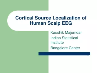
Cortical Source Localization of Human Scalp EEG. Kaushik Majumdar Indian Statistical Institute Bangalore Center. Cortical Basis of Scalp EEG. Baillet et al., IEEE Sig. Proc. Mag., Nov 2001, p. 16.

E N D
Cortical Source Localization of Human Scalp EEG Kaushik Majumdar Indian Statistical Institute Bangalore Center
Cortical Basis of Scalp EEG Baillet et al., IEEE Sig. Proc. Mag., Nov 2001, p. 16.
Mountcastle, Brain, 120:701-722, 1997. Six Layer Cortex
Source Localization in Two Parts • Part I : Forward Problem • Part II : Inverse Problem
Forward Problem : Schematic Head Model EEG Channels Source Scalp Skull Brain
Dipole Source Model (parametric model) Distributed Source Model (nonparametric model) Source Models
Majumdar, IEEE Trans. Biomed. Eng., vol. 56(4), p. 1228 – 1235, 2009. Distributed Source Model
Kybic et al., Phys. Med. Biol., vo. 51, p. 1333 – 1346, 2006 Forward Calculation • Poisson’s equation in the head
Hallez et al., J. NeuroEng. Rehab., 2007, open access. http://www.jneuroengrehab.com/content/4/1/46 Published Conductivity Values
Hallez et al., J. NeuroEng. Rehab., 2007, open access. http://www.jneuroengrehab.com/content/4/1/46 6 Parameter Dipole Geometry
Potential at any Single Scalp Electrode Due to All Dipoles r is the position vector of the scalp electrode rdip - i is the position vector of the ith dipole di is the dipole moment of the ith dipole
Generalization V = GD + n G is gain matrix, n is additive noise.
EEG Gain Matrix Calculation For detail of potential calculations see Geselowitz, Biophysical J., 7, 1967, 1-11.
Boundary Elements Method for Distributed Source Model • If on the complement of a smooth surface then can be completely determined by its values and the values of its derivatives on that surface.
Hallez et al., J. NeuroEng. Rehab., 2007, open access. http://www.jneuroengrehab.com/content/4/1/46 Nested Head Tissues SKULL BRAIN SCALP
Kybic, et al., IEEE Trans. Med. Imag., vol. 24(1), p. 12 – 28, 2005. Representation Theorem Ω be a connected, open, bounded subset of R3 and ∂Ω be regular boundary of Ω. u : R3- ∂Ω → R is harmonic and r|u(r)| < ∞, r(∂u/∂r) = 0, then if p(r) = ∂nu(r) the following holds:
Representation Theorem (cont) I is the identity operator and
Representation Theorem (cont) ∂nG means n.▼G, where n is normal to an interfacing head tissue surface.
Justification • Holes in the skull (such as eyes) account for up to 2 cm of error in source localization. • The closer a source is to the cortical surface the more its effect tends to smear. • If size of mesh triangles is of the order of the gaps between the surfaces the errors go up rapidly. • Implemented in OpenMeeg – an open source software (openmeeg.gforge.inria.fr/ ).
Kybic, et al., IEEE Trans. Med. Imag., vol. 24(1), p. 12 – 28, 2005. Distributed Source : Gain Matrix
Gain Matrix (cont) Gain matrix is to be obtained by multiplying several matrices A, one for each layer in the single layer formulation.
Hallez et al., J. NeuroEng. Rehab., 2007, open access. http://www.jneuroengrehab.com/content/4/1/46 Finite Elements Method
Further Reading on FEM • Awada et al., “Computational aspects of finite element modeling in EEG source localization,” IEEE Trans. Biomed. Eng., 44(8), pp. 736 – 752, Aug 1997. • Zhang et al., “A second-order finite element algorithm for solving the three-dimensional EEG forward problem,” Phys. Med. Biol., vol. 49, pp. 2975 – 2987, 2004.
Inverse Problem : Peculiarities • Inverse problem is ill-posed, because the number of sensors is less than the number of possible sources. • Solution is unstable, i.e., susceptible to small changes in the input values. Scalp EEG is full of artifacts and noise, so identified sources are likely to be spurious.
Mattout et al., NeuroImage, vol. 30(3), p. 753 – 767, Apr 2006 Weighted Minimum Norm Inverse V = BJ + E, V is scalp potential, B is gain matrix and E is additive noise. Minimize U(J) = ||V – BJ||2Wn + λ||J||2Wp λ is a regularization positive constant between 0 and 1.
Geometric Interpretation ||V-BJ||2Wn ||J||2Wp Convex combination of the two terms with λ very small. minU(J)
Derivation U(J) = ||V – BJ||2Wn + λ||J||2Wp = <Wn(V – BJ), Wn(V – BJ)> + λ<WpJ, WpJ> ΔJU(J) = 0 implies (using <AB,C> = <B,ATC>) J = CpBT[BCpBT + Cn]-1V where Cp = (WTpWp)-1 and Cn = λ(WTnWn)-1.
Different Types • When Cp = Ip (the p x p identity matrix) it reduces to classical minimum norm inverse solution. • In terms of Bayesian notation we can write E(J|B) = CpBT[BCpBT + Cn]-1V. On this expectation maximization algorithm can be readily applied.
Types (cont) • If we take Wp as a spatial Laplacian operator we get the LORETA inverse formulation. • If we derive the current density estimate by the minimum norm inverse and then standardize it using its variance, which is hypothesized to be due to the source variance, then that is called sLORETA.
Types (cont) • Recursive – MUSIC Mosher & Leahy, IEEE Trans. Biomed. Eng., vol. 45(11), p. 1342 – 1354, Nov 1998.
Low Resolution Brain Electromagnetic Tomography (LORETA) Pascual-Marqui et al., Int. J. Psychophysiol., vol. 18, p. 49 – 65, 1994.
Standardized Low Resolution Brain Electromagnetic Tomography (sLORETA) U(J) = ||V – BJ||2 + λ||J||2 Ĵ = TV, where T = BT[BBT + λH]+, where H = I – LLT/LTL is the centering matrix. Pascual-Marqui at http://www.uzh.ch/keyinst/NewLORETA/sLORETA/sLORETA-Math02.htm
sLORETA (cont) Ĵ is estimate of J, A+ denotes the Moore-Penrose inverse of the matrix A, I is n x n identity matrix where n is the number of scalp electrodes, L is a n dimensional vector of 1’s. Hypothesis : Variance in Ĵ is due to the variance of the actual source vector J. Ĵ = BT[BBT + λH]+BJ.
If # Source = # Electrodes = n • B and BT both will be n x n identity matrix. with λ = 0
http://www.uzh.ch/keyinst/loreta.htm sLORETA Result
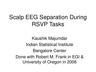
Single Trial Source Localization • Averaging signals across the trials to increase the SNR cannot be done.
Generated using OpenMeeg in INRIA Sophia Antipolis in 2008. Cortical Sources
Generated using OpenMeeg in INRIA Sophia Antipolis in 2008. Localization by MN
Majumdar, IEEE Trans. Biomed. Eng., vol. 56(4), p. 1228 – 1235, 2009. Clustering
Trial Selection • Identify the time interval. • Identify channels. • Calculate cumulative signal amplitude in those channels. • Sort trials according to the decreasing amplitude.