Download

1 / 42
430 likes | 744 Vues
ME 259 Heat Transfer Lecture Slides III. Dr. Gregory A. Kallio Dept. of Mechanical Engineering, Mechatronic Engineering & Manufacturing Technology California State University, Chico. Transient Conduction. Reading: Incropera & DeWitt Chapter 5. Introduction.

E N D
ME 259Heat TransferLecture Slides III Dr. Gregory A. Kallio Dept. of Mechanical Engineering, Mechatronic Engineering & Manufacturing Technology California State University, Chico ME 259
Transient Conduction Reading: Incropera & DeWitt Chapter 5 ME 259
Introduction • Transient = Unsteady (time-dependent ) • Examples • Very short time scale: hot wire anemometry (< 1 ms) • Short time scale: quenching of metallic parts (seconds) • Intermediate time scale: baking cookies (minutes) • Long time scale – daily heating/cooling of atmosphere (hours) • Very long time scale: seasonal heating/cooling of the earth’s surface (months) ME 259
Governing Heat Conduction Equation • Assuming k = constant, • For 1-D conduction (x) and no internal heat generation, • Solution, T(x,t) , requires two BCs and an initial condition ME 259
The Biot Number • The Biot number is a dimensionless parameter that indicates the relative importance of of conduction and convection heat transfer processes: • Practical implications of Bi << 1: objects may heat/cool in an isothermal manner if • they are small and metallic • they are cooled/heated by natural convection in a gas (e.g., air) ME 259
The Lumped Capacitance Method (LCM) • LCM is a viable approach for solving transient conduction problems when Bi<<1 • Treat system as an isothermal, homogeneous mass (V) with uniform specific heat (cp) • For suddenly imposed, uniform convection (h, T) boundary conditions, solution yields: where ME 259
General LCM • LCM can be applied to systems with convection, radiation, and heat flux boundary conditions and internal heat generation (see eqn. 5.15 for ODE) • Forced convection, h = constant • Natural convection, h = C(T-T)1/4 • Radiation (eqn. 5.18) • Convection and radiation (requires numerical integration) • Forced convection with constant surface heat flux or internal heat generation (eqn. 5.25) (Note that the Biot number must be redefined when effects other than convection are included) ME 259
Spatial Effects (Bi 0.1) • LCM not valid since temperature gradient within solid is significant • Need to solve heat conduction equation with applied boundary conditions • 1-D transient conduction “family” of solutions: • Uniform, symmetric convection applied to plane wall, long cylinder, sphere (sections 5.4-5.6) • Semi-infinite solid with various BCs (section 5.7) • Superposition of 1-D solutions for multidimensional conduction (section 5.8) ME 259
Convection Heat Transfer: Fundamentals Reading: Incropera & DeWitt Chapter 6 ME 259
The Convection Problem • Newton’s law of cooling (convection) • “h” is often the controlling parameter in heat transfer problems involving fluids; knowing its value accurately is important • h can be obtained by • theoretical derivation (difficult) • direct measurement (time-consuming) • empirical correlation (most common) • Theoretical derivation is difficult because • h is dependent upon many parameters • it involves solving several PDEs • it usually involves turbulent fluid flow, for which no unified modeling approach exists ME 259
Average Convection Coefficient • Consider fluid flow over a surface: • Total heat rate: • If h = h(x), then ME 259
The Defining Equation for h • The thermal boundary layer: • From Fourier’s law of conduction: • Setting qconv = qcond andsolving for h: ME 259
Determination of • Need to find T(x,y) within fluid boundary layer, then differentiate and evaluate at y = 0 • T(x,y) is obtained by solving the following conservation equations: • Mass (continuity) ……. Eqn (6.25) • Momentum (x,y) ……. Eqn (6.26, 6.27) • Thermal Energy …….. Eqn (6.28a,b) • Solution of these four coupled PDEs yields the velocity components (u,v), pressure (p), and temperature (T) • Exact solution is only possible for laminar flow in simple geometries ME 259
Boundary Layer Approximations • Because the velocity and thermal boundary layer thicknesses are typically very small, the following BL approximations apply: • The BL approximations with the additional assumptions of steady-state, incompressible flow, constant properties, negligible body forces, and zero energy generation yield a simpler set of conservation equations given by eqns. (6.31-6.33). ME 259
Boundary Layer Similarity Parameters • BL equations are normalized by defining the following dimensionless parameters: where L is the characteristic length of the surface and V is the velocity upstream of the surface • The resulting normalized BL equations (Table 6.1) produce the following unique dimensionless groups: • Note: all properties are those of the fluid ME 259
Boundary Layer Similarity Parameters, cont. • Recall the defining equation for h: • The normalized temperature gradient at the surface is defined as the Nusselt number, which provides a dimensionless measure of the convection heat transfer: ME 259
The Nusselt Number • The normalized BL equations indicate that • Since the Nusselt number is a normalized surface temperature gradient, its functional dependence for a prescribed geometry is • Recalling that the average convection coefficient results from an integration over the entire surface, the x* dependence disappears and we have: ME 259
Physical Significance of the Reynolds and Prandtl Numbers • Reynolds number (VL/) represents a ratio of fluid inertia forces to fluid viscous shear forces • small Re: low velocity, low density, small objects, high viscosity • large Re: high velocity, high density, large objects, low viscosity • Prandtl number (cp/k) represents the ratio of momentum diffusion to heat diffusion in the boundary layer. • small Pr:relatively large thermal boundary layer thickness (t > ) • large Pr: relatively small thermal boundary layer thickness (t < ) • Note that Pr is a (composite) fluid property that is commonly tabulated in property tables ME 259
The Reynolds Analogy • The BL equations for momentum and energy are similar mathematically and indicate analogous behavior for the transport of momentum and heat • This analogy allows one to determine thermal parameters from velocity parameters and vice-versa (e.g., h-values can be found from viscous drag values) • The heat-momentum analogy is applicable in BLs when dp*/dx* 0 (turbulent flow is less sensitive to this) • The modified Reynolds analogy states • where Cf is the skin friction coefficient ME 259
Turbulence • Turbulence represents an unsteady flow, characterized by random velocity, pressure, and temperature fluctuations in the fluid due to small-scale eddies • Turbulence occurs when the Reynolds number reaches some critical value, determined by the particular flow geometry • Turbulence is typically modeled with eddy diffusivities for mass, momentum, and heat • Turbulent flow increases viscous drag, but may actually reduce form drag in some instances • Turbulent flow is advantageous in the sense of providing higher h-values, leading to higher convection heat transfer rates ME 259
Forced Convection Heat Transfer – External Flow Reading: Incropera & DeWitt Chapter 7 ME 259
The Empirical Approach • Design an experiment to measure h • steady-state heating • transient cooling, Bi<<1 • Perform experiment over a wide range of test conditions, varying: • freestream velocity (u ) • type of fluid (, ) • object size (L) • Reduce data in terms of Reynolds, Nusselt, and Prandtl ME 259
The Empirical Approach, cont. • Plot reduced data, NuL vs. ReL, for each fluid (Pr): • Develop an equation curve-fit to the data; a common form is typically: < m < 1 < n < 0.01 < C < 1 ME 259
Flat Plate in Parallel, Laminar Flow (the Blasius Solution) • Assumptions: • steady, incompressible flow • constant fluid properties • negligible viscous dissipation • zero pressure gradient (dp/dx = 0) • Governing equations ME 259
Blasius Solution, cont. • Similarity solution, where a similarity variable () is found which transforms the PDEs to ODEs: • Blasius derived: ME 259
Empirical Correlations • Flat Plate in parallel flow: Section 7.2 • Cylinder in crossflow: Section 7.4 • Sphere: Section 7.5 • Flow over banks of tubes: Section 7.6 • Impinging jets: Section 7.7 ME 259
Forced Convection Heat Transfer – Internal Flow Reading: Incropera & DeWitt Chapter 8 ME 259
Review of Internal (Pipe) Flow Fluid Mechanics • Flow characteristics • Reynolds number • Laminar vs. turbulent flow • Mean velocity • Hydrodynamic entry region • Fully-developed conditions • Velocity profiles • Friction factor and pressure drop ME 259
Pipe Reynolds Number • um is mean velocity, given by • Reynolds number for circular pipes: • Reynolds number determines flow condition: • ReD < 2300 : laminar • 2300 < ReD < 10,000 : turbulent transition • ReD > 10,000 : fully turbulent ME 259
Pipe Friction Factor • Darcy friction factor, f, is a dimensionless parameter related to the pressure drop: • For laminar flow in smooth pipes, • For turbulent flow in smooth pipes, • good for3000 < ReD < 5x10⁶ • For rough pipes, use Moody diagram (Figure 8.3) or Colebrook formula (given in most fluid mechanics texts) ME 259
Pressure Drop and Power • For fully-developed flow, dp/dx is constant; so the pressure drop ( p) in a pipe of length L is • The pump or fan power (Wp) required to overcome this pressure drop is • where p is the pump or fan efficiency ME 259
Thermal Characteristics of Pipe Flow • Thermal entry region • Thermally fully-developed conditions • Mean temperature • Newton’s law of cooling ME 259
Newton’s Law of Cooling & Mean Temperature • The absence of a fixed freestream temperature necessitates the use of a mean temperature, Tm, in Newton’s law of cooling: • Tm is the average fluid temperature at a particular cross-section based upon the transport of thermal (internal) energy, Et: • Unlike T , Tm is not a constant in the flow direction; it will increase in a heating situation and decrease in a cooling situation. ME 259
Fully-Developed Thermal Conditions • While the fluid temperature T(x,r) and mean temperature Tm(x) never reach constant values in internal flows, a dimensionless temperature difference does - and this is used to define the fully-developed condition: • the following must also be true: • therefore, from the defining equation for h: i.e., h = constant in the fully-developed region ME 259
Pipe Surface Conditions • There are two special cases of interest, that are used to approximate many real situations: 1) Constant surface temperature (Ts = const) 2) Constant surface heat flux (q”s = const) ME 259
Review of Energy Balance Results • For any incompressible fluid or ideal gas pipe flow, 1) For constant surface heat flux, 2) For constant surface temperature, 3) For constant ambient fluid temperature, ME 259
Convection Correlations for Laminar Flow in Circular Pipes • Fully-developed conditions with Pr > 0.6: • Note that these correlations are independent of Reynolds number ! • All properties evaluated at (Tmi+Tmo)/2 • Entry region with Ts = const and thermal entry length only (i.e., Pr >> 1 or unheated starting length): • combined entry length correlation given by eqn. (8.57) in text ME 259
Convection Correlations for Turbulent Flow in Circular Pipes • Fully-developed conditions, smooth wall, q”s = const or Ts = const • Dittus-Boelter equation - fully turbulent flow only (ReD > 10,000) and 0.7 < Pr < 160 • NOTE: should not be used for transitional flow or flows with large property variation ME 259
Convection Correlations for Turbulent Flow in Circular Pipes, cont. • Sieder-Tate equation - fully tubulent flow (ReD > 10,000),very wide range of Pr (0.7 - 16,700), large property variations • Gnielinski equation - transitional and fully-turbulent flow (3000 < ReD < 5x10⁶), wide range of Pr (0.5 - 2000) • f given on a previous slide (eqn. 8.21) ME 259
Convection Correlations for Turbulent Flow in Circular Pipes, cont. • Entry Region • Recall that the thermal entry region for turbulent flow is relatively short, I.e.,only 10 to 60D • Thus, fully-developed correlations are generally valid if L/D > 60 • For 20 < L/D < 60, Molki & Sparrow suggest • Liquid Metals (Pr << 1) • Correlations for fully-developed turbulent pipe flow are given by eqns. (8.65), (8.66) ME 259
Convection Correlations for Noncircular Pipes • Hydraulic Diameter, Dh • where: Ac = flow cross-sectional area P = “wetted” perimeter • Laminar Flows (ReDh < 2300) • use special NuDhrelations • rectangular & triangular pipes: Table 8.1 • annuli: Table 8.2, 8.3 • Turbulent Flows (ReDh > 2300) • use regular pipe flow correlations with ReD and NuD based upon Dh ME 259
Heat Transfer Enhancement • A variety of methods can be used to enhance the convection heat transfer in internal flows; this can be achieved by • increasing h, and/or • increasing the convection surface area • Methods include • surface roughening • coil spring insert • longitudinal fins • twisted tape insert • helical ribs ME 259