Searching the search space graph
590 likes | 929 Vues
Searching the search space graph. 171: Class 3. Recap: State-Space Formulation. Intelligent agents: problem solving as search Search consists of state space operators start state goal states The search graph A Search Tree is an effective way to represent the search process

Searching the search space graph
E N D
Presentation Transcript
Searching the search space graph 171: Class 3
Recap: State-Space Formulation • Intelligent agents: problem solving as search • Search consists of • state space • operators • start state • goal states • The search graph • A Search Tree is an effective way to represent the search process • There are a variety of search algorithms, including • Depth-First Search • Breadth-First Search • Others which use heuristic knowledge (in future lectures)
Uninformed search strategies • Uninformed: While searching you have no clue whether one non-goal state is better than any other. Your search is blind. You don’t know if your current exploration is likely to be fruitful. • Various blind strategies: • Breadth-first search • Uniform-cost search • Depth-first search • Iterative deepening search
Breadth-first search • Expand shallowest unexpanded node • Fringe: nodes waiting in a queue to be explored, also called OPEN • Implementation: • fringe is a first-in-first-out (FIFO) queue, i.e., new successors go at end of the queue. Is A a goal state?
Breadth-first search • Expand shallowest unexpanded node • Implementation: • fringe is a FIFO queue, i.e., new successors go at end Expand: fringe = [B,C] Is B a goal state?
Breadth-first search • Expand shallowest unexpanded node • Implementation: • fringe is a FIFO queue, i.e., new successors go at end Expand: fringe=[C,D,E] Is C a goal state?
Breadth-first search • Expand shallowest unexpanded node • Implementation: • fringe is a FIFO queue, i.e., new successors go at end Expand: fringe=[D,E,F,G] Is D a goal state?
Example BFS
B C A G S D F E Example: Map Navigation S = start, G = goal, other nodes = intermediate states, links = legal transitions
A B C S G D E F Initial BFS Search Tree S D A D B E E C Note: this is the search tree at some particular point in in the search.
Breadth First Search Tree (BFS) S D A B A E D S E E C F S B B (Use the simple heuristic of not generating a child node if that node is a parent to avoid “obvious” loops: this clearly does not avoid all loops and there are other ways to do this)
What is the Complexity of Breadth-First Search? • Time Complexity • assume (worst case) that there is 1 goal leaf at the RHS • so BFS will expand all nodes = 1 + b + b2+ ......... + bd = O (bd) • Space Complexity • how many nodes can be in the queue (worst-case)? • at depth d there are bdunexpanded nodes in the Q = O (bd) • Time and space of number of generated nodes is O (b^(d+1)) d=0 d=1 d=2 G d=0 d=1 d=2 G
Examples of Time and Memory Requirements for Breadth-First Search Depth of Nodes Solution Expanded Time Memory 0 1 1 millisecond 100 bytes 2 111 0.1 seconds 11 kbytes 4 11,111 11 seconds 1 megabyte 8 108 31 hours 11 giabytes 12 1012 35 years 111 terabytes Assuming b=10, 1000 nodes/sec, 100 bytes/node
Depth-First-Search (*) 1. Put the start node s on OPEN 2. If OPEN is empty exit with failure. 3. Remove the first node n from OPEN and place it on CLOSED. 4. If n is a goal node, exit successfully with the solution obtained by tracing back pointers from n to s. 5. Otherwise, expand n, generating all its successors attach to them pointers back to n, and put them at the top of OPEN in some order. 6. Go to step 2.
1 2 3 7 4 6 5 8 9 10 11 12 13 14 15 Breadth-First Search (BFS) Properties • Complete • Solution Length: optimal • (Can) expand each node once (if checks for duplicates) • Search Time: O(bd) • Memory Required: O(bd) • Drawback: requires exponential space
Depth-first search • Expand deepest unexpanded node • Implementation: • fringe = Last In First Out (LIPO) queue, i.e., put successors at front Is A a goal state?
Depth-first search • Expand deepest unexpanded node • Implementation: • fringe = LIFO queue, i.e., put successors at front queue=[B,C] Is B a goal state?
Depth-first search • Expand deepest unexpanded node • Implementation: • fringe = LIFO queue, i.e., put successors at front queue=[D,E,C] Is D = goal state?
Depth-first search • Expand deepest unexpanded node • Implementation: • fringe = LIFO queue, i.e., put successors at front queue=[H,I,E,C] Is H = goal state?
Depth-first search • Expand deepest unexpanded node • Implementation: • fringe = LIFO queue, i.e., put successors at front queue=[I,E,C] Is I = goal state?
Depth-first search • Expand deepest unexpanded node • Implementation: • fringe = LIFO queue, i.e., put successors at front queue=[E,C] Is E = goal state?
Depth-first search • Expand deepest unexpanded node • Implementation: • fringe = LIFO queue, i.e., put successors at front queue=[J,K,C] Is J = goal state?
Depth-first search • Expand deepest unexpanded node • Implementation: • fringe = LIFO queue, i.e., put successors at front queue=[K,C] Is K = goal state?
Depth-first search • Expand deepest unexpanded node • Implementation: • fringe = LIFO queue, i.e., put successors at front queue=[C] Is C = goal state?
Depth-first search • Expand deepest unexpanded node • Implementation: • fringe = LIFO queue, i.e., put successors at front queue=[F,G] Is F = goal state?
Depth-first search • Expand deepest unexpanded node • Implementation: • fringe = LIFO queue, i.e., put successors at front queue=[L,M,G] Is L = goal state?
Depth-first search • Expand deepest unexpanded node • Implementation: • fringe = LIFO queue, i.e., put successors at front queue=[M,G] Is M = goal state?
A B C S G D E F Search Method 2: Depth First Search (DFS) S D A B D E C Here, to avoid repeated states assume we don’t expand any child node which appears already in the path from the root S to the parent. (Again, one could use other strategies) F D G
Depth-First-Search (*) 1. Put the start node s on OPEN 2. If OPEN is empty exit with failure. 3. Remove the first node n from OPEN and place it on CLOSED. 4. If n is a goal node, exit successfully with the solution obtained by tracing back pointers from n to s. 5. Otherwise, expand n, generating all its successors attach to them pointers back to n, and put them at the top of OPEN in some order. 6. Go to step 2.
What is the Complexity of Depth-First Search? d=0 • Time Complexity • assume (worst case) that there is 1 goal leaf at the RHS • so DFS will expand all nodes(m is cutoff) =1 + b + b2+ ......... + b^m = O (b^m) • Space Complexity • how many nodes can be in the queue (worst-case)? • at depth l < d we have b-1 nodes • at depth d we have b nodes • total = (m-1)*(b-1) + b = O(bm) d=1 d=2 G d=0 d=1 d=2 d=3 d=4
Repeated states • Failure to detect repeated states can turn a linear problem into an exponential one!
Solutions to repeated states S B • Method 1 • do not create paths containing cycles (loops) • Method 2 • never generate a state generated before • must keep track of all possible states (uses a lot of memory) • e.g., 8-puzzle problem, we have 9! = 362,880 states • Method 1 is most practical, work well on most problems S B C C C S B S State Space Example of a Search Tree
Properties of depth-first search A • Complete? No: fails in infinite-depth spaces Can modify to avoid repeated states along path • Time?O(bm) with m=maximum depth • terrible if m is much larger than d • but if solutions are dense, may be much faster than breadth-first • Space?O(bm), i.e., linear space! (we only need to remember a single path + expanded unexplored nodes) • Optimal? No (It may find a non-optimal goal first) B C
Comparing DFS and BFS • Same worst-case time Complexity, but • In the worst-case BFS is always better than DFS • Sometime, on the average DFS is better if: • many goals, no loops and no infinite paths • BFS is much worse memory-wise • DFS is linear space • BFS may store the whole search space. • In general • BFS is better if goal is not deep, if infinite paths, if many loops, if small search space • DFS is better if many goals, not many loops, • DFS is much better in terms of memory
Iterative Deepening (DFS) • Every iteration is a DFS with a depth cutoff. Iterative deepening (ID) • i = 1 • While no solution, do • DFS from initial state S0 with cutoff i • If found goal, stop and return solution, else, increment cutoff Comments: • ID implements BFS with DFS • Only one path in memory • BFS at step i may need to keep 2i nodes in OPEN
Properties of iterative deepening search • Complete? Yes • Time?O(bd) • Space?O(bd) • Optimal? Yes, if step cost = 1 or increasing function of depth.
Iterative Deepening Time (DFS) • Time: • BFS time is O(bn) • b is the branching degree • ID is asymptotically like BFS • For b=10 d=5 d=cut-off • DFS = 1+10+100,…,=111,111 • IDS = 123,456 • Ratio is
Comments on Iterative Deepening Search • Complexity • Space complexity = O(bd) • (since its like depth first search run different times) • Time Complexity • 1 + (1+b) + (1 +b+b2) + .......(1 +b+....bd) • = O(bd) (i.e., asymptotically the same as BFS or DFS in the worst case) • The overhead in repeated searching of the same subtrees is small relative to the overall time • e.g., for b=10, only takes about 11% more time than BFS • A useful practical method • combines • guarantee of finding an optimal solution if one exists (as in BFS) • space efficiency, O(bd) of DFS • But still has problems with loops like DFS
Bidirectional Search • Idea • Simultaneously search forward from S and backwards from G • stop when both “meet in the middle” • need to keep track of the intersection of 2 open sets of nodes • What does searching backwards from G mean • need a way to specify the predecessors of G • this can be difficult, • e.g., predecessors of checkmate in chess? • what if there are multiple goal states? • what if there is only a goal test, no explicit list? • Complexity • time complexity is best: O(2 b(d/2)) = O(b (d/2)), worst: O(bd+1) • memory complexity is the same
Uniform Cost Search • Expand lowest-cost OPEN node (g(n)) • In BFS g(n) = depth(n) • Requirement • g(successor)(n)) g(n)
6 1 A D F 1 3 2 4 8 S G B E 1 20 C Find minimum cost path The graph above shows the step-costs for different paths going from the start (S) to the goal (G). On the right you find the straight-line distances. Use uniform cost search to find the optimal path to the goal.
Uniform cost search 1. Put the start node s on OPEN 2. If OPEN is empty exit with failure. 3. Remove the first node n from OPEN and place it on CLOSED. 4. If n is a goal node, exit successfully with the solution obtained by tracing back pointers from n to s. 5. Otherwise, expand n, generating all its successors attach to them pointers back to n, and put them at the end of OPEN in order of shortest cost • Go to step 2.