Download
1 / 66
680 likes | 1.4k Vues
MVN- based Multilayer Feedforward Neural Network (MLMVN) and a Backpropagation Learning Algorithm. Introduced in 2004-2007. MLMVN.

E N D
MVN- based Multilayer Feedforward Neural Network(MLMVN)and a Backpropagation Learning Algorithm Introduced in 2004-2007
MLMVN • I. Aizenberg and C. Moraga, "Multilayer Feedforward Neural Network based on Multi-Valued Neurons and a Backpropagation Learning Algorithm", Soft Computing, vol. 11, No 2, January, 2007, pp. 169-183. • I. Aizenberg, D. Paliy, J. Zurada, and J. Astola, "Blur Identification by Multilayer Neural Network based on Multi-Valued Neurons", IEEE Transactions on Neural Networks, vol. 19, No 5, May 2008, pp. 883-898.
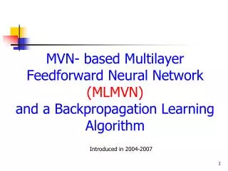
1 2 N MVN- based Multilayer Feedforward Neural Network Hidden layers Output layer
MLMVN: Key Properties • Derivative-free learning algorithm based on the error- correction rule • Self-adaptation of the learning rate for all the neurons • Much faster learning than the one for other neural networks • A single step is always enough to adjust the weights for the given set of inputs independently on the number of hidden and output neurons • Better recognition/prediction/classification rate in comparison with other neural networks, neuro-fuzzy networks and kernel based techniques including SVM
MLMVN: Key Properties • MLMVN can operate with both continuous and discrete inputs/outputs, as well as with the hybrid inputs/outputs: • continuous inputs discrete outputs • discrete inputs continuous outputs • hybrid inputs hybrid outputs
- a desired output of the kth neuron from the mth (output) layer - an actual output of the kth neuron from the mth (output) layer - the network error for the kth neuron from output layer - the error for the kth neuron from output layer -the number of all neurons on the previous layer (m-1, to which the error is backpropagated) incremented by 1 A Backpropagation Derivative- Free Learning Algorithm
The error for the kth neuron from the hidden (jth) layer, j=1, …, m-1 -the number of all neurons on the previous layer (previous to j, to which the error is backpropagated) incremented by 1 A Backpropagation Derivative- Free Learning Algorithm The error backpropagation:
A Backpropagation Derivative- Free Learning Algorithm Correction rule for the neurons from the mth (output) layer (kth neuron of mth layer):
A Backpropagation Derivative- Free Learning Algorithm Correction rule for the neurons from the 2nd through m-1st layer (kth neuron of the jth layer (j=2, …, m-1):
A Backpropagation Derivative- Free Learning Algorithm Correction rule for the neurons from the 1st hidden layer:
Criteria for the convergence of the learning process Learning should continue until either minimum MSE/RMSE criterion will be satisfied or zero-error will be reached
λ is a maximum possible MSE for the training data N is the number of patterns in the training set is the network square error for the sth pattern MSE criterion
λ is a maximum possible RMSE for the training data N is the number of patterns in the training set is the network square error for the sth pattern RMSE criterion
MLMVN Learning: Example Suppose, we need to classify three vectors belonging to three different classes: Classes are determined in such a way that the argument of the desired output of the network must belong to the interval
MLMVN Learning: Example Thus, we have to satisfy the following conditions: , where is the actual output. . and for the mean square error
11 x1 21 x2 12 MLMVN Learning: Example Let us train the 21 MLMVN (two hidden neurons and the single neuron in the output layer
MLMVN Learning: Example The training process converges after 7 training epochs. Update of the outputs:
Simulation Results: Benchmarks All simulation results for the benchmark problems are obtained using the network with n inputs nS1 containing a single hidden layer with S neurons and a single neuron in the output layer: Hidden layer Output layer
Two Spirals Problem:cross-validation (training of 98 points and prediction of the rest 96 points) The prediction rate is stable for all the networks from 2261 till 2401: 68-72% The prediction rate of 74-75% appears 1-2 times per 100 experiments with the network 2401 The best known result obtained using the Fuzzy Kernel Perceptron (Nov. 2002) is 74.5%, But it is obtained using more complicated and larger network
Mackey-Glass time series prediction Mackey-Glass differential delay equation: . The task of prediction is to predict from
Mackey-Glass time series prediction Training Data: Testing Data:
Mackey-Glass time series prediction RMSE Training: RMSE Testing:
Mackey-Glass time series prediction Testing Results: Blue curve – the actual series; Red curve – the predicted series
Mackey-Glass time series prediction The results of 30 independent runs:
Mackey-Glass time series prediction Comparison of MVN to other models: • MLMVN outperforms all other networks in: • The number of either hidden neurons or supporting vectors • Speed of learning • Prediction quality
Real World Problems: Solving Using MLMVN
Generation of the Genetic Code using MLMVN • I. Aizenberg and C. Moraga, "The Genetic Code as a Function of Multiple-Valued Logic Over the Field of Complex Numbers and its Learning using Multilayer Neural Network Based on Multi-Valued Neurons", Journal of Multiple-Valued Logic and Soft Computing, No 4-6, November 2007, pp. 605-618
Genetic code • There are exactly four different nucleic acids: Adenosine (A), Thymidine (T), Cytidine (C) and Guanosine (G) • Thus, there exist 43=64 different combinations of them “by three”. • Hence, the genetic code is the mapping between the four-letter alphabet of the nucleic acids (DNA) and the 20-letter alphabet of the amino acids (proteins)
Genetic code as a multiple-valued function • Let be the amino acid • Let be the nucleic acid • Then a discrete function of three variables • is a function of a 20-valued logic, which is partially defined on the set of four-valued variables
Genetic code as a multiple-valued function • A multiple-valued logic over the field of complex numbers is a very appropriate model to represent the genetic code function • This model allows to represent mathematically those biological properties that are the most essential (e.g., complementary nucleic acids AT; G C that are stuck to each other in a DNA double helix only in this order
AT; GC DNA double helix The complementary nucleic acids are always stuck to each other in pairs
G G R C E W AT; GC D M N I K T A F Y L Q V H S A T P C Representation of thenucleic acidsandamino acids The complementary nucleic acids are located such that A=1; G=i T= -A= -1 and C= - G = -i All amino acids are distributed along the unit circle in the logical way, to insure their closeness to those nucleic acids that form each certain amino acid
Generation of the genetic code • The genetic code can be generated using MLMVN341 (3 inputs, 4 hidden neurons and a single output neuron – 5 neurons) • There best known result for the classical backpropagation neural network is generation of the code using the network 312220 (32 neurons)
Blurred Image Restoration (Deblurring) and Blur Identification by MLMVN
Blurred Image Restoration (Deblurring) and Blur Identification by MLMVN • I. Aizenberg, D. Paliy, J. Zurada, and J. Astola, "Blur Identification by Multilayer Neural Network based on Multi-Valued Neurons", IEEE Transactions on Neural Networks, vol. 19, No 5, May 2008, pp. 883-898.
Problem statement: capturing • Mathematically a variety of capturing principles can be described by the Fredholm integral of the first kind • where x,t ℝ2, v(t) is a point-spread function (PSF) of a system, y(t) is a function of a real object and z(x) is an observed signal. • Photo • Tomography • Microscopy
Image deblurring: problem statement • Mathematically blur is caused by the convolution of an image with the distorting kernel. • Thus, removal of the blur is reduced to the deconvolution. • Deconvolution is an ill-posedproblem,which results in the instability of a solution. The best way to solve it is to use some regularization technique. • To use any kind of regularization technique, it is absolutely necessaryto know the distorting kernel corresponding to a particular blur: so it is necessary to identify the blur.
Image deblurring: problem statement The observed image given in the following form: where “*” denotes a convolution operation, y is an image, υ is point-spread function of a system (PSF) , which is exactly a distorting kernel, and ε is a noise. In the continuous frequency domain the model takes the form: where is a representation of the signal z in the Fourier domain and denotes a Fourier transform.
Blur Identification • We use MLMVN to recognize Gaussian, motion and rectangular (boxcar) blurs. • We aim to identify simultaneously both blur (PSF), and its parameters using a single neural network.
Considered PSF PSF in time domain PSF in frequency domain Gaussian Motion Rectangular
Considered PSF The Gaussian PSF: is a parameter (variance) The uniform linear motion: his a parameter (the length of motion) The uniform rectangular: his a parameter (the size of smoothing area)
Degradation in the frequency domain: True Image Rectangular Horizontal Motion Vertical Motion Gaussian Images and log of their Power Spectra
Training Vectors • We state the problem as a recognition of the shape of V, which is a Fourier spectrum of PSF vand its parameters from the Power-Spectral Density, whose distortions are typical for each type of blur.
Training Vectors The training vectors are formed as follows: for • LxLis a size of an image • the length of the pattern vector isn= 3L/2-3
Examples of training vectors True Image Gaussian Rectangular Horizontal Motion Vertical Motion