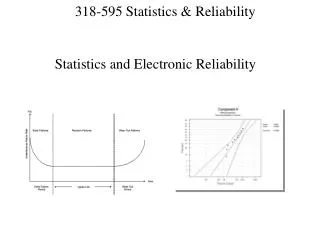
Statistics and Electronic Reliability
Statistics and Electronic Reliability. Printed Circuit Board Assemblies. Review of Printed Circuit Board Technology 3 Basic Types of PCB-Component Assembly Technology Thru Hole (TH) using prepackaged devices Surface Mount (SMT) using prepackaged devices

Statistics and Electronic Reliability
E N D
Presentation Transcript
Printed Circuit Board Assemblies Review of Printed Circuit Board Technology • 3 Basic Types of PCB-Component Assembly Technology • Thru Hole (TH) using prepackaged devices • Surface Mount (SMT) using prepackaged devices • Micro-electronic using bare die and prepackaged devices • 3 Basic Types of PCB Substrates (fabs) • Rigid copper-epoxy laminate PCB (single, dual up to ~40 layers) • Alumina, Alum Nitride or other ceramic materials (up to ~20 layers) • Flexible Substrate (Polyimide-Copper, up to 8 layers) • Surface Metalization Finishes • HASL – Hot Air Solder Leveling (Eutectic SnPb Surfaces, lowest cost) • ENIG – Electroless Ni – Immersion Au (flatter for wirebonding, BGA, ACF) • IAg – Immersion Silver (co-deposited with organics to reduce reactivity, replacement for ENIG) • Electroplated Finishes – NiAu over Cu, not always possible depending on circuit
Causes of Electronic Systems Failure Reliability ofElectronic Circuits • Failures can generally be divided between intrinsic or extrinsic failures • Intrinsic failures- Inherent in the component technology • Electromigration (semiconductors, substrates) • Contact wear (relays, connectors, etc) • Contamination effects- e.g. channeling, corrosion, leakage • CTE mismatch and other Interconnection joint fatigue • Extrinsic failures- External stress to the components • ESD or Electrostatic discharge energy • Electrical overstress (over voltage, overload, overheat) • Shock (Sudden Mechanical Impact) • Vibration (Periodic Mechanical G force) • Humidity or condensable water • Package Mishandling, Bending, Shear, Tensile • Many “random” and infantile failures of components are due to extrinsic failures • Wearout failures are usually due to intrinsic failures
PCB Assembly Failure Mechanisms • Stresses & Major Factors • Thermal Excursion and Cycling • Coef of Thermal Expansion (CTE) mismatches • Package and Substrate Sizes (Larger is worse) • # of Interconnects on Package (More is worse) • Solder joint geometry including cracks, voids and skew • Mechanical Shock and Vibration • Mass of Components and Overall Assembly • Height of Component Center of Mass (COG) • Thickness, Rigidity and Support Pts of PCB • Solder joint geometry including cracks, voids and skew
Printed Circuit Board Assemblies CTE Mismatches in PCB Assemblies Si Die CTE = 2.8e-6/C Gold CTE = 14.2e-6/C5 – 15 μ in. NiAu Pad Thin Epoxy Solder Mask Nickel CTE = 13.4e-6/C> ~100 μ in. Copper FR4 Laminate CTE = ~20e-6/C Copper CTE = 16.5e-6/C> ~1.2 mil SnPb Eutectic Solder Joint CTE = ~25e-6/C
PCB Assembly Failure Mechanisms • Stresses & Major Factors - continued • Electrochemical • Usage environment incl ambient temp & humidity • Usage environment incl corrosive materials, salts, etc • Maximum electrical field (induced by spacing, voltage on PCB) • Ionic Cleanliness of PCB over/under solder mask and other coatings • Cations: Including Lithium, Sodium, Ammonium, Potassium, Magnesium and Calcium. Many companies limit each individual cation contribution to be less than 0.2ug/cm2 and the combined total of all cations to be less than 0.50ug/cm2. • Anions: Most Destructive Includes Fluoride, Chloride, Nitride, Bromide, Sulfate, and Phosphates. Many companies limit each individual anion contribution to be less than 0.1ug/cm2 and the combined total of all anions to be less than 0.25ug/cm2. • Weak Organic Acids: May include Acetate, Formate, Succinate, Glutamate, Malate, Methane Sulfonate (MSA), Phthalate, Phosphate, Citrate and Adipic Acids. Many companies limit the combined total of all weak organic acids to be less than or equal to ~0.75ug/cm2 • Ion cleanliness is tested per IPC TM-650 2.3.28 using Ion Chromatography for high reli assemblies. IPC-6012/15 mandate a total ionic cleanliness of less than 1.56ug/cm2 = 10ug/in2.
Ionic Test Methods for PCBs Resistivity of Solvent Extract (ROSE) Test Method IPC-TM-650 2.3.25The ROSE test method is used as a process control tool (rinse) to detect the presence of bulk ionics. The IPC upper limit is set at 10.0 mg/in2 .(1.56ug/cm2) This test method provides no evidence of a correlation value with modified ROSE testing or ion chromatography. This test is performed using an ionograph or similar style ionics testing unit that detects total ionic contamination, but does not identify specific ions present. Non destructive test. Modified Resistivity of Solvent Extract (Modified ROSE)The modified ROSE test method involves a thermal extraction. The PCB is exposed in a solvent solution at a predetermined temperature for a specified time period. This process draws the ions present on the PCB into the solvent solution. The solution is tested using an ionograph-style test unit. The results are reported as bulk ions present on the PCB per square inch, similar to the standard ROSE method above. Can be destructive. Ion Chromatography IPC-TM-650 2.3.28This test method involves a thermal extraction similar to the modified ROSE test. After thermal extraction, the solution is tested using various standards in an ion chromatographic test unit. The results indicate the individual ionic species present and the level of each ion species per unit area. This test is an excellent way to pinpoint likely process steps which are leaving residual contaminants that can lead to early reliability failures. Destructive test.
Specifying Warranty: Must Understand Reliability of Product (1, 5 yrs, etc) • Life of Product should be less than wear out failure mode period • Bathtub Reli Curve: (Failure Rate vs Time) Area under curve = total failures Infantile Period ~ Constant Failure Rate Minimize or Precipitate using ESS in factory Warranty Period Using ESS Warranty Period
25 22 20 18 15 12 10 8 5 2 0 1.238 1.240 1.242 1.244 Basic Statistics and Reliability Statistics
n X S i i = 1 m = = X n n 2 S ( X - X ) i s i = 1 = s = n - 1 Basic Statistics Review Example: The following data represents the amount of time it takes 7 people to do a 355 exam problem. X = 2, 6, 5, 2 ,10, 8, 7 in min. n = 7 where X = index notation for each individual. where n = 7 people i i whereS X = Sum of the individual times where X and m = Average or Mean Calculate the mean(average): Equation i n = 7 people Mean:X = (2+6+5+2+10+8+7)/7 = 5.7 minutes where s = s = Standard Deviation Sum or Variance Calculate the standard deviation: Equation Step 1 Step 2 (Xi - X) (Xi - X) 2-5.7= -3.7 13.69 6-5.7= .3 .09 5-5.7 = -.7 .49 2-5.7 = -3.7 13.69 10-5.7 = 4.3 18.49 8-5.7 = 2.3 5.29 7-5.7 = 1.3 1.69 S(Xi - X) = 53.43 Step 4 Definition: Range = Max - Min Median = Middle number when arranged low to high Mode = Most common number This Example: Range = 10 - 2 = 8 minutes Median = 6 minutes Mode = 2 minutes 2 53.43 Square each one Then Add All s = s = 7 - 1 Standard Deviation: = 2.98 minutes s = s 2 Step 3 Std Deviation is a measure of the inherent spread in the data
25 22 20 18 15 12 10 8 5 2 0 1.238 1.240 1.242 1.244 Bar Chart or Histogram Provides a visual display of data distribution Shape of Distribution May be Key to Issues • Normal (Bell Shaped) • Uniform (Flat) • Bimodal (Mix of 2 Normal Distributions) • Skewed left or right • Total number of bins is flexible but usually no more than 10 • By using an infinite number of bins, resultant curve is a distribution • Use T-Test to Compare Means, F-Test to Compare Variances
Target Specification Limit 3s Histogram vs Spec Limits Area under curve Is probability of failure 1s 66807ppm PPM = Part per Million Defects Z is the number of Std Devs between the Mean and the spec limit. The higher the value of Z, the lower the chance of producing a defect Z = 3s Much Less Chance of Failure 1s 3.4ppm* * Assumes Z is 4.5 long term Normal Distribution Z = 6s
(with ± 1.5 shift) PPM 1,000,000 IRS - Tax Advice (phone-in) (140,000 PPM) Restaurant Bills 100,000 Doctor Prescription Writing Payroll Processing 10,000 • Average Company Airline Baggage Handling 1,000 100 10 Best-in-Class 1 6 2 3 4 5 7 Z Domestic Airline Flight Fatality Rate (0.43 PPM) Examples of Fault/Failure Rates on The Sigma Scale
Shift and Drift Short Term Capability Snapshots of the Product Over time, a “typical” product process may shift or drift by ~ 1.5 . . . also called “short-term capability” . . . reflects ‘within group’ variation Time 1 Time 2 Time 3 Time 4 Actual Sustained Capability of the Process . . . also called “long-term capability” . . . reflects ‘total process’ variation LSL T USL Two Challenges: Center the Process and Eliminate Variation!
100 % 75 % 50 % 25 % 0 % 100 % 75 % 50 % 25 % 0 % Statistics Example: IPC Workmanship Classes: Solder Volume, Shape, Placement Control • High Reliability Electronic Products: Includes the equipment for commercial and military products where continued performance or performance on demand is critical. Equipment downtime cannot be tolerated, and functionality is required for such applications as life support or missile systems. Printed board assemblies in this class are suitable for applications where high levels of assurance are required and service is essential. • Requirement for Aero-Space, Certain Military, Certain Medical • Dedicated Service Electronic Products: Includes communications equipment, sophisticated business machines, instruments and military equipment where high performance and extended life is required, and for which uninterrupted service is desired but is not critical. Typically the end-use environment would NOT cause failures. • Requirement for High Eng Telecom, COTS Military, Medical • General Electronic Products: Includes consumer products, some computer and peripherals, as well as general military hardware suitable for applications where cosmetic imperfections are not important and the major requirement is function of the completed printed board assembly. Min PTH Vertical Fill: Class 2 = 75% Class 3 = 100% Ref: IPC-A-610, IPC-JSTD-001
BGA Void Size and Locations,Uniform Void Position Distribution, Varying Diameter Sampling_Grid Position Model Solder_Joint_Radius Void_Distance Void_Radius S Void_Solder Interface Distance S = Shell Potential for Early Life Failure (ELFO) if S < D/10 = (solder_joint_radius)/10 S =Shell = solder_joint_radius – (void_distance + void_radius)
CLASS 1 - GOOD Solder Joint_Radius: 0.225 mm Void_Radius: 0.135 mm Void_Area: 36% of Joint Area Failure criteria: D/10 P(D<10) = 81.11 % CLASS 2 - BETTER Solder Joint_Radius: 0.225 mm Void_Radius: 0.1013 mm Void_Area: 20% of Joint Area Failure criteria: D/10 P(D<10) = 52.21 % CLASS 3 - BEST Solder Joint_Radius: 0.225 mm Void_Radius: 0.0675 mm Void_Area: 9% of Joint Area Failure criteria: D/10 P(D<10) = 27.00 %
Class vs Shell Size Relative Probabilities~ 2x more likely to exceed D/10 threshold with Class 2 vs Class 3 S = Shell Depth
Exponential Distributions = Reliability = Time
Definitions • l General Failure Rate Variable: Recall the Bathtub Curve- Failure Rate (l) vs. Time behavior • For CONSTANT FAILURE RATES – Exponential Distribution Applies and R(t) = (Reliability at Time t) = Probability that a system will not fail for a time period “t,” assuming constant failure rate; • R(t) = e-lt, Note: lis in failures/time, and t is time • Note: At T=0, R(0)=1.0 (100%) lFIT = FITs = Failures per 109 hours MTBF (years) = 1x10⁹ / (lFIT * 8766 hours /year ) lMTBF = 1/MTBF = 1/Mean time between failure in hours R(t) = e-lt, Note: lMTBF in hr-1 and t in hr
Definitions l General Failure Rate Variable: For CONSTANT FAILURE RATES – Exponential Distribution Applies and R(t) = (Reliability at Time t) = Probability that a system will not fail for a time period “t,” assuming constant failure rate; R(t) = e-lt, Note: lis in failures/time, and t is time Note: At T=0, R(0)=1.0 (100%) F(t) = (UnReliability at Time t or Failures at Time t) = Fraction of population that has failed at Time t, probability that a given system will fail for a time period “t,” assuming constant failure rate; F(t) = 1-e-lt, Note: lis in failures/time, and t is time Note: At T=0, F(0)=0.0 (0%)
Weibull or 2 Parameter Distributions For VARYING FAILURE RATES – Weibull Distribution Applies and R(t) = (Reliability at Time t) = Probability that a system will not fail for a time period “t,”; • R(t) = e-(t/h)b, Note: his the dimensionless scale parameter (stretches) • b is the shape or slope parameter • Note: At T=0, R(0)=1.0 (100%) • Relationship of Weibull parameters to Failure Rate • = (/h)(t/h)-1 • R(t) = e-(t/h)b • F(t) = 1-e-(t/h)b
Typical Reliability Plot using Weibull Dist • = (/h)(t/h)-1 • F(t) = 1-e-(t/h)b F(t) = (1 – R(t))100% Time to Failure(s)
Typical Reliability Plot assuming Weibull Dist • = (/h)(t/h)-1 • R(t) = e-(t/h)b • F(t) = 1-e-(t/h)b Time to failure plot using Weibull tool Decreasing Failure Rates <1 Increasing Failure Rates >1 The Bathtub Curve Constant Failure Rates =1 Exponential Distribution Failure Rate, Weibull slope indicates where the product may be on the bathtub curve. Early Life Wear out Useful Life Time
Intro to Reliability Evaluation • Basic Series Reli Method of an Electronic System: Component 1 l1 Component 2 l2 Component i li Component N lN • Each component has an associated reliability l • The System Reli lss is the sum of all the component l • lss = Sli • Reli l is expressed in “FITs” failure units • x FIT = x Failures/109 hours • Note: 109 hours = 1 Billion Hours
Example • An electronics assembly product has an MTBF of 20000 hours; constant failure rate • What is the probability that a given unit will work continuously for one year? • Reliability R(t) = e-lt • l = 1/MTBF = 1/20000 hr • l = 0.00005 hr-1 (Failure rate) • t = 8766 hours (1 year) • R(1yr) =e-(8766/20,000) = 0.65 = 65% • In other words, the Mean Time Between failures is 20,000 hours or about 2.3 years • But … 35% of the units would likely fail in the first year of operation. • Remember, after 1 MTBF R(t) = 1/e = 0.368 = 36.8% of population without failure
Intro to Reliability Evaluation • Basic Series Reli Method of an Electronic System: Component 1 R1 Component 2 R2 Component i Ri Component N RN • Each component also has an associated reliability R • The System R is the product of all the component R • R = P Ri • Recall, Reli R is a probability (0 to 1) expressed in percent
Reliability R Flowdown Example Drive System, needs R= 0.9 at 10 years System Level Power supply R = 0.94 Subsystem Level Motor R = 0.97 Control Card R = 0.99 Component Level Part R=0.9999 Part R=0.9999 Part R=0.9999 Part R=0.9999 Part R=0.9999 Part R=0.999 Part R=0.999
Reliability Requirements Flowdown- Example • Customer’s need: Meet R=90%@ 10 years • Partition requirements to subsystems • Based on engineering analysis, experience, vendor data, parts count, etc. • Allocation: • Rsystem = Rpower * Rcontroller * Rmotor • Rsystem = 0.94 * 0.99 * 0.97 = 0.90 • Each of the 3 subsystems should in turn be allocated to components
MTBF Example • An electronics product team has a goal of warranty cost which requires that a • Minimum reliability after 1 year be 99% or higher, R(1yr) >= 0.99. Assume Constant • Failure Rates. • What MTBF should the team work towards to meet the goal? Recall Equations: R = e -lt and MTBF = 1/l Solve for MTBF: MTBF = 1/ l = 1/ {(-1/t) * ln R }, R = 0.99, t = 8766 hrs MTBF >= 872,000 hours (99.5 yrs) ! What is your product warranty cost goal expressed as an R(t)?: Answer:What is the scrap or repair cost of a given % of failures during the warranty period? Need to know, annual production, and an assumed R(t). Good products have less than 1% annualized warranty cost as a percentage of the total contribution margin for that product.
Some Typical Stresses • Environmental: Temp, Humid, Pressure, Wind, Sun, Rain • Mechanical: Shock, Vibration, Rotation, Abrasion • Electrical: Power Cycle, Voltage Tolerance, Load, Noise • ElectroMagnetic: ESD, E-Field, B-Field, Power Loss • Radiation: Xray (non-ionizing), Gamma Ray (ionizing) • Biological: Mold, Algae, Bacteria, Dust • Chemical: Alchohol, Ph, TSP, Ionic
Intro to Reliability Estimation • Each l may be impacted by other factors or stresses, p: • Some commonly used factors • pT = Temperature Stress Factor • pV = Electrical Stress Factor • pE = Environmental Factor • pQ = Quality Factor • Overall Component l = lB * pT * pV * pE * pQ Where lB = Base Failure Rate for Component
Reliability Prediction Methods/Standards • Bellcore (TR-TSY-000332): • Developed by Bell Communications Research for general use in electronics industry although geared to telecom. • Highest Stress Factor is Electrical Stress • Data based upon field results, lab testing, analysis, device mfg data and US Military Std 217 • Stress Factors include environment, quality, electrical, thermal • US Military Handbook 217F: • Developed by the US Department of Defense as well as other agencies for use by electronic manufacturers supplying to the military • Describes both a “parts count” method as well as a “parts stress” method • Data is based upon lab testing including highly accelerated life testing (HALT) or highly accelerated stress testing (HAST) • Stress factors include environment and quality
Reliability Prediction Methods/Standards • HRD4 (Hdbk of Reliability Data for Comp, Issue 4): • Developed by the British Telecom Materials and Components Center for use by designers and manufacturers of telecom equipment • Stress factors include thermal as well as environment, quality with quality being dominant • Standard describes generic failure rates based upon a 60% confidence interval around data collected via telecom equipment field performance in the UK • CNET: • Developed by the French National Center of Telecommunications • Similar to HRD4, stress factors include thermal as well as environment and dominant quality • Data is based upon field experience of French commercial and military telecom equipment
Reliability Prediction Methods/Standards • Siemens AG (SN29500): • Developed by Siemens for internal uniform reliability predictions • Stress factors include thermal and electrical however thermal dominates • Standard describes failures rates based upon applications data, lab testing as well as US Mil Std 217 • Components are classified into technology groups each with tuned reliability model
Reliability Prediction • Basic Series Reli Method of an Electronic System: Component 1 l1 Component 2 l2 Component i li Component N lN • Above Reliability Prediction Model is flawed because; • Components may not have constant reliability rates l • lss = Sli • Component applications, stresses, etc may not be well matched by the method used to model reliability • Not all component failures may lead to a system failure • Example: A bypass capacitor fails as an open circuit
595 Standard Failure Rates in FIT (Data is not accurate in all cases)
595 Standard Failure Rates in FIT (Data is not accurate in all cases)
595 Standard Stress Factors • Factor Definitions (may not represent standard models) • pT = Temperature Stress Factor = e[Ta/(Tr-Ta)] – 0.4 • Where Ta = Actual Max Operating Temp, Tr = Rated Max Op Temp, Tr>Ta • pV = Cap/Res/Transistor Electrical Stress Factor = e[(Va)/Vr-Va]-2.0 • Where Va = Actual Max Operating Voltage, Vr = Abs Max Rated Voltage, Vr>Va • pE = Environmental (Overall) Factor >>> • Indoor Stationary = 1.0 • Indoor Mobile = 1.5 • Outdoor Stationary = 2.0 • Outdoor Mobile = 2.5 • Automotive = 3.0 • pQ = Quality Factor (Parts and Assembly) • Mil Spec/Range Parts = 0.75 • 100 Hr Powered Burn In = 0.75 • Commercial Parts Mfg Direct = 1.0 • Commerical Parts Distributor = 1.25 • Hand Assembly Part = 3.0
Part Max Tr Max Vr pT pV pE pQ C1 105C 50V 2.082 0.186 2.5 1.25 C2 105C 50V 2.082 0.186 2.5 1.25 C3 85C 15V 3.773 0.223 2.5 1.25 C4 125C 50V 1.548 0.151 2.5 1.25 R1 120C 20V 1.643 0.232 2.5 1.25 R2 150C 6V 1.249 0.549 2.5 1.25 Zener Diode 100C N/A 2.318 1.0 2.5 1.25 Op Amp 125C 36V 1.548 1.0 2.5 1.25 74HCT14 125C 7V 1.548 1.649 2.5 1.25 LED 85C N/A 3.773 1.0 2.5 1.25 Example: Method A, 0-50C Ambient, Outdoor Mobile, Distributor Components +5VDC C1 0.1uf 50V Polyester +12VDC C4 0.1uf 50V Ceramic +5VDC LED Vf=1.5V R1 2KW 1/4W Brand A Metal Film Vin BPLR OP AMP R2 150W 1/4W Brand B Metal Film C2 0.1uf 50V Polyester 74HCT14 5V 1W Zener C3 10uf 15V Electrolytic -12VDC lTotal 10.29 10.29 552.2 1.46 0.83 1.50 23.18 67.73 217.77 106.16 991.37 Fits 115.1 Years
Stress Factors Drive Simple: 595 Standard Deratings • Resistors, Potentiometers <= 50% maximum power • Caps/Res <= 60% maximum working voltage • Transistors <= 50% maximum working voltage • Note: Most discrete devices as well as linear IC’s have parameters which will vary with temperature which is expressed as Tc (temp coefficient). Typically a delta or percent of change per deg C from ambient.
MTBF Data Input Sheet for e-Reliability.com COST: $500 per report System / Equipment Name:Assembly Name:Quantity of this assembly:Parts List Number:Environment:Select One Of : GB, GF, GM, NS, NU, AIC, AIF, AUC, AUF, ARW, SF, MF, ML, or CLParts Quality:Select Either: Mil-Spec or Commercial/BellcoreQuantity Description---------- Bipolar Integrated Circuits IC / Bipolar, Digital 1-100 Gates IC / Bipolar, Digital 101-1000 Gates IC / Bipolar, Digital 1001-3000 Gates IC / Bipolar, Digital 3001-10000 Gates IC / Bipolar, Digital 10001-30000 Gates IC / Bipolar, Digital 30001-60000 Gates IC / Bipolar, Linear 1-100 Transistors IC / Bipolar, Linear 101-300 Transistors IC / Bipolar, Linear 301-1K Transistors IC / Bipolar, Linear 1001-10K Transistors, etc. EXAMPLE: Actual Reli Tool Input List of components, their number, Environment conditions, components quality
Example Reliability calculation using actual MIL-HDBK-217F Failure rate of a Metal Oxide Semiconductor (MOS) can be expressed as Parameters are listed in MIL Data base. Temperature factor is modeled using Arrhenius type Eqn
Example Reliability report --------------------------------------------------------------------------------------- | | | | | Failure Rate in | | | | | | Parts Per Million Hours | | Description/ | Specification/ | Quantity | Quality |-------------------------| | Generic Part Type | Quality Level | | Factor | | | | | | | (Pi Q) | Generic | Total | | | | | | | | |=====================|================|==========|=========|============|============| | Integrated Circuit/ | Mil-M-38510/ | 16 | 1.00 | 0.07500 | 1.20000 | | Bipolar, Digital | B | | | | | | 30001-60000 Gates | | | | | | | | | | | | | | Integrated Circuit/ | Mil-M-38510/ | 8 | 1.00 | 0.01700 | 0.13600 | | Bipolar, Linear | B | | | | | | 101-300 Transistors | | | | | | | | | | | | | | Diode/ | Mil-S-19500/ | 2 | 2.40 | 0.00047 | 0.00226 | | Switching | JAN | | | | | | | | | | | | | | | | | | | | Diode/ | Mil-S-19500/ | 4 | 2.40 | 0.00160 | 0.01536 | | Voltage Ref./Reg. | JAN | | | | | | (Avalanche & Zener) | | | | | | | | | | | | | | Transistor/ | Mil-S-19500/ | 4 | 2.40 | 0.00007 | 0.00067 | | NPN/PNP | JAN | | | |
Parts Count Method Reliability Prediction Drawbacks • Prediction Methods not always effective in representing future reality of a product. Tend to be pessimistic, however they are generally inaccurate. • Best utilized for design comparison and order of magnitude reliability prediction (must use same methods for comparisons) • Single Stress Factors must be employed to represent a composite average or worst case of the population. Difficult to predict average stress levels, peak stress levels • Methods give an overall average failure rate, one dimensional • Time to failure distributions (Weibull) are two dimensional describing infantile failures as well as end of life failures • Reli growth using actual stress testing is a much more effective process (however also more expensive approach) • MIL-STD-217F Notice 2 was the last revision of this long used standard (Jan 1995), No further releases planned.