Satellite orbits
Satellite orbits. Satellite orbits. Satellites and their orbits GEO LEO Special orbits (e.g., L 1 ) Satellite sensor types Whiskbroom Pushbroom Pixel size calculation. Launch. Launch of Aura satellite July 15, 2004 Vandenberg, CA . ~96% fuel ~4% payload.

Satellite orbits
E N D
Presentation Transcript
Satellite orbits • Satellites and their orbits • GEO • LEO • Special orbits (e.g., L1) • Satellite sensor types • Whiskbroom • Pushbroom • Pixel size calculation
Launch Launch of Aura satellite July 15, 2004 Vandenberg, CA ~96% fuel ~4% payload Recent launch failures: Orbiting Carbon Observatory (OCO) Glory
Satellite orbits • Determined by Kepler’s Laws • Planets (and satellites) move in elliptical orbits • The square of the orbital period is proportional to the cube of the semi-major axis of the orbit • Altered by atmospheric drag, gravity of Sun and Moon • Orbital period = time taken for satellite to circle the Earth • P0= orbital period, a = semi-major axis of ellipse (satellite altitude + Earth radius [~6380 km]), G = Gravitational constant, M = mass of Earth (GM = 3.986×10¹⁴ m3 s-2) • NB. This assumes that the Earth is spherically symmetric (it isn’t) Launch of Aura satellite July 15, 2004 Vandenberg, CA
Geostationary orbits (GEO) Launch of Aura satellite July 15, 2004 Vandenberg, CA • Special type of geosynchronous orbit • Orbital period = period of Earth’s rotation • 86164 seconds for a sidereal day • Circular orbit around the equator with zero inclination • Orbit is stationary with respect to a location on the Earth • Advantages: high temporal resolution, always visible (e.g., weather forecasting, communications); ~5-15 minutes • Disadvantages: cost, lower spatial resolution than polar-orbiting sensors, poor coverage of high latitudes (>55ºN/S)
GOES Super Rapid-Scan http://cimss.ssec.wisc.edu/goes/blog/archives/6849
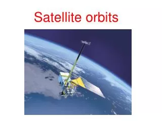
Polar or Low-Earth orbits (LEO) Launch of Aura satellite July 15, 2004 Vandenberg, CA
Polar or Low-Earth orbits (LEO) Launch of Aura satellite July 15, 2004 Vandenberg, CA • Useful altitude range: ~500-2000 km above Earth’s surface • Constrained by atmospheric friction and van Allen belts (high flux of energetic charged particles) • Because Earth is not spherical, polar orbits precess (rotate) about the Earth’s polar axis • Sun-synchronous orbits precess at the same rate that the Earth orbits the Sun • Altitudes ~700-800 km, periods of 98-102 minutes • 14-15 orbits per day • e.g., NOAA-X satellites (US), MetOp (Europe) • Advantages: high spatial resolution, polar coverage • Disadvantages: low temporal resolution (at low latitudes)
LEO repeat cycles Launch of Aura satellite July 15, 2004 Vandenberg, CA If Earth makes an integral number of rotations in the time taken for the satellite to complete an integral number of orbits, the sub-satellite track repeats exactly. e.g., NASA Aura satellite (705 km altitude) has a 16-day (233 orbit) repeat cycle
LEO polar coverage Launch of Aura satellite July 15, 2004 Vandenberg, CA LEO orbits converge at the Poles, providing higher temporal resolution
LEO at low inclination Launch of Aura satellite July 15, 2004 Vandenberg, CA NASA Tropical Rainfall Measuring Mission (TRMM) – 35º inclination, 403 km altitude http://trmm.gsfc.nasa.gov
LEO spacecraft constellations NASA’s A-Train
L1 Lagrange point 1.5 million kilometers from Earth!
Space junk GEO LEO 18,000 manmade objects and counting!
Space-borne imaging systems • Cross-track scanners • Whiskbroom scanners • Pushbroom sensors • http://www.ssec.wisc.edu/sose/pirs_activity.html
FOV – IFOV - GIFOV FOV: Field of View IFOV: Instantaneous FOV GIFOV: Ground-projected IFOV
Cross-track scanner • Scans back and forth across the sensor’s swath • Scans each ground-resolution cell (pixel) one-by-one • Instantaneous field of view (IFOV) of sensor determines pixel size • Satellite moves along the orbital track as sensor scans across-track • Divided into ‘line’ and ‘whiskbroom’scanners • Disadvantages: moving parts, expensive, short pixel ‘dwell time’, pixel distortion
Whiskbroom scanner Landsat Multi-spectral Scanner (MSS)
Dwell time (cross-track) • Time period over which sensor collects photons from an individual ground-resolution cell • Determines signal-to-noise ratio (SNR) • Given by [scan time per line]/[# of cells per line] • Example: • Landsat sensor with 30×30 m pixel, 185 km swath width; spacecraft velocity = ~7.5 km/s • [along-track pixel size] / [orbital velocity] • [swath width] / [cross-track pixel size]
Along-track scanner (pushbroom) • Linear array of detectors aligned across-track (e.g., CCD) • Image built up by satellite movement in flight direction (no scanning mirror) • 2D detector arrays can acquire multi-spectral or hyperspectral data • Optics disperse wavelengths across detector array
Dwell time (pushbroom) • Time period over which sensor collects photons from an individual ground-resolution cell • Determines signal-to-noise ratio (SNR) • Denominator = 1 in equation below in this case • Example: • Different sensitivities and responses in each detector pixel can cause ‘striping’ in pushbroom sensor data • [along-track pixel size] / [orbital velocity] • [swath width] / [cross-track pixel size]
Satellite viewing geometry Nadir Sub-satellite point
Pixel size calculation • β = Instantaneous Field of View (IFOV) • H = satellite altitude • Pixel size = 2 H tan (β/2) • Example: • Aura satellite altitude = 705 km • OMI (Ozone Monitoring Instrument) • OMI telescope IFOV in flight direction = 1º • Pixel size = 1410 tan (0.5) = 12.3 km • NB: strictly speaking, this is the Ground-projected IFOV (GIFOV) – pixel size could be different H β Pixel size
Field of View (FOV) • FOV = 2 H tan (scan angle + β/2) • H = satellite altitude • Example: • Aura satellite altitude = 705 km • OMI telescope swath FOV = 115º • FOV = 1410 tan (57.5) = 2213 km • But this assumes a flat Earth… θ H FOV/2
Field of View (FOV) • Use Law of Sines • Note ambiguity for sin β • Swath width = 2d α h rs d β re re ϕ