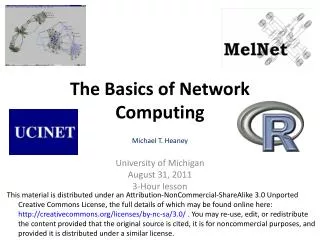
The Basics of Network Computing
The Basics of Network Computing. Michael T. Heaney University of Michigan August 31, 2011 3-Hour lesson. Plan for the Afternoon. Choosing a Network Program Working with Network Data Basic network statistics Visualization. Principal Tasks of Network Computing. Visualization of Networks

The Basics of Network Computing
E N D
Presentation Transcript
The Basics of Network Computing Michael T. Heaney University of Michigan August 31, 2011 3-Hour lesson
Plan for the Afternoon Choosing a Network Program Working with Network Data Basic network statistics Visualization
Principal Tasks of Network Computing Visualization of Networks Calculation of Descriptive Statistics Advanced Network Analysis (e.g., ERGM) When considering which statistical package to use, consider which of the above tasks your work will focus on.
UCINet Operates well in the familiar windows environment, but may be difficult to use with Apple computers. Allows calculation of most standard network statistics, but is less adept at handling advanced analysis (e.g., ERGM). Point-and-click approach is relatively easy to learn, but it can be a bit clunky. Available here: http://www.analytictech.com/ucinet/download.htm
Statnet in R Operates well in both Windows and Apple computing environments Performs both basic and advanced network analyses Users can develop own network analysis routines Steep learning curve Available here: http://statnetproject.org/
Some Other Packages MelNet – Specializes in Exponential Random Graph Models. Available: http://www.sna.unimelb.edu.au/ Pajek – Specializes in large network analysis. Available: http://vlado.fmf.uni-lj.si/pub/networks/pajek/ SoNIA– Visualizing Dynamic Networks. Available: http://www.stanford.edu/group/sonia/ And more…..
UCINet A good place to start training even if you are going to shift to another program.
Importing Data Simplest approach is to read an Excel file. Open UCINet Click on Spreadsheet Icon File Open Excel Files Filename.xlsx In this case, open Hrmatrix.xlsx Save as UCINET 7 dataset Note the creation of two files filename.##h and filename. ##d – you will need both of these files in order to use UCINET data.
Data List Files A good alternative when you are working with large data sets Create using a simple text file: dl nr = 1945 nc = 525, format = edgelist2, labels embedded data: 10270716051 Communist 10270716049 UFPJ 10270716048 BrooklynPeace 10270716045 BrooklynPeace 10270716045 UFPJ
Read a Data List File Data Import Text File DL… Contact_Network_Data OK
More Varied DL Formats for Data Best to learn this on your own using UCINet help Help Help Topics DL
Basic Data Analysis – Density Network Cohesion (new) Density Overall Hrmatrix
Compute Density with Two-Mode Data Network 2-Mode networks 2-mode Cohesion Input 2-mode incidence matrix OK
Basic Network Analysis – Centrality Network Centrality and Power Multiple Measures (old)
Using Your Centrality Data in Statistical Analysis Spreadsheet File Open Centrality Save as type Excel Excel File Open
Compute Centrality with Two-Mode Data Network 2-Mode Networks 2-Mode Centrality Input 2-mode matrix Contact_Network_Data.##h OK
Convert Two-Mode Data to One-Mode Data Data Affiliations (2-mode to 1-mode) Input data … Contact_Network_Data Which mode Column [for this particular example]
Using Your Affiliation Data Note that your new one-mode data (i.e., affiliation data) has been saved as a new file: Contact_Network_Data-ColAff You can conduct all network analysis on this dataset Let’s look at it: Spreadsheet File Open Contact_Network_Data-ColAff OK Note that your cells make are counts of affiliations, which is why we call this affiliation data
Dichotomizing Data Are data may be valued, but we may preferred that they be dichotomous Transform Dichotomize Contact_Network_Data-ColAff Our output will now have only 1s and 0s
Basic Visualization Visualize Netdraw File Open Ucinet Dataset Network Choose File
Refine Visualization Open Ucinet dataset Attribute data HRattributes Properties Lines Arrow Heads Visible Off Properties Nodes Symbols Size Attribute Based Age Properties Nodes Symbols Shape Attribute Based English_language Layout Graph-Theoretic Layout Spring Embedding OK
Visualizing Contact Network Data UCINet Spreadsheet File Open Excel Files Hybrid_Variable.xlsx File Save As UCINet 7 dataset Hybrid_Variable Visualize Netdraw File Open Ucinet Dataset Network Contact_Network_Data-ColAff File Open Ucinet Dataset Attribute data Hybrid_Variable
Visualizing Contact Network Data – Continued Click on delete isolates buttons Layout Graph Theoretic Layout Spring Embedding (You may need to do this twice) Analysis Components OK
Visualizing Contact Network Data – Continued Click on MC button to look at main component only Turn off labels, arrow heads Repeat spring embedding Properties Lines Size Tie Strength 1 to 10 Properties Nodes Symbols Shape Attribute Based Select Attribute Hybrid Variable OK Click a node Choose label visible
Visualizing Contact Network Data – Continued Analysis Subgroups Factions 2 (or 3 or 4) Go!
Next Steps Multiplex Visualizations Three Dimensional Visualizations Advanced analysis Exponential Random Graph Models