CHAPTER 2: DEMAND, SUPPLY & MARKET EQUILIBRIUM
460 likes | 1.68k Vues
CHAPTER 2: DEMAND, SUPPLY & MARKET EQUILIBRIUM. 1.1 Introduction: Market Mechanism Principles 1.2 Demand 1.3 Supply 1.4 Market Equilibrium 1.5 Change in SS & DD 1.6 SS/DD Analysis Example. Microeconomics scope for UBEA 1013 Economics. Output (Product) Market. DD & SS Interaction.

CHAPTER 2: DEMAND, SUPPLY & MARKET EQUILIBRIUM
E N D
Presentation Transcript
CHAPTER 2: DEMAND, SUPPLY & MARKET EQUILIBRIUM 1.1 Introduction: Market Mechanism Principles 1.2 Demand 1.3 Supply 1.4 Market Equilibrium 1.5 Change in SS & DD 1.6 SS/DD Analysis Example
Microeconomics scope for UBEA 1013 Economics Output (Product) Market DD & SS Interaction Consumers (Demand) Firms (Supply) Changes in DD / SS: Equilibrium Price & Quantity Production Supplier surplus Factors effect SS Elasticity Market structure Utility (excluded) Consumer surplus Factors effect DD Elasticity Input (Factor) Market
1.1 Introduction: Market Mechanism Principles Market & the circulation flow Economics decision-making units Demand & supply interaction
1.2 Demand Definition: “Demand” can be defined as the purchase of product. ONE household / individual ALL Household / Individual Market demand Household / individual demand Demand curve (graph) Demand function (equation)
Demand curve (graph): Demand function (equation): Quantity of X demanded, QdX = f (PX; PY, I, preference, and others) Factor effecting quantity demanded Factor effecting demand
Demand function (equation): Quantity of X demanded, QdX = f (PX; PY, I, preference, and others) 1 Law of Demand: – negative, or inverse relationship between price & quantity – movement along demand curve – change in quantity demanded • Relationship of products: • – substitution or complement product: (PY) • – normal, luxury or inferior products: (I) • (ii) Shift of DD curve: (PY, I, preference, and others) • – (later section) new equilibrium price & quantity 2
Law of Demand: 1 Figure 2.3: Price & Quantity Demanded: The Law of Demand Law of Demand: – negative, or inverse relationship – movement along demand curve – change in quantity demanded Why?: Due to the income constraint and utility interaction. Exception?: Giffin product.
2 Shift of DD curve & Relationship of products: PY change: Substitute – Substitutes are products that can replace one another – Positive relationship between PY and demand for X (the substitute product): When (PY) increases, demand for X increases. – Examples: Coffee & tea; Coca-cola & Pepsi Cola Law of demand Substitution product
Shift of DD curve & Relationship of products: PY change:Complement – Complement are products that are consumed together – Negative relationship between PY and demand for Z (the complement product): When (PY) decreases, demand for Z increases. – Examples: Car & petrol; coffee & sugar Law of demand Complement product
Shift of DD curve & Relationship of products: Income change: Normal Product I ↑ – Demand increase when income increase – Examples: Cloth & movie Income change: Luxury Product – Same effect as normal product but demand increase more when income increase – Examples: luxury car. Normal product I ↑ Income change: Inferior Product – Low quality products (potato & secondhand cloth) – Income increase, demand decrease (able to buy better quality product). Inferior product
Shift of DD curve & Relationship of products: Necessity Product? Insignificant product? – Their consumption did not effect much by change in income. Their consumption is only a very small percentage of total income. – The demand curve did not shift (or shift too little that we can ignore) – Examples: salt
Shift of DD curve & Relationship of products: Other factors: Taste / preference – Demand increase when taste / preference towards the product increase (DD curve shift to the left) – Examples: low fat item & fashion Other factors: Expected future price – Demand increase when Future price of product is expected to increase (DD curve shift to the left) – Examples: If petrol price to increase from 12am tomorrow, demand for petrol increase immediately (today). Other factors: Increase of buyer – Increase in number of buyer, increase demand (DD curve shift to the left) … continue
1.3 Supply Definition: “Supply” can be defined as selling of product. ONE firm ALL firms Market supply Individual (firm) supply Supply curve (graph) Supply function (equation)
Supply curve (graph): Supply function (equation): Quantity of X supplied, QSX = f (PX; K, L, technology, PY and others) Factor effecting quantity supplied Factor effecting supply
Supply function (equation): Quantity of X demanded, QSX = f (PX; K, L, technology, PY and others) 1 Law of Supply: – positive relationship between price & quantity – movement along supply curve – change in quantity supplied Shift of SS curve: (K, L, technology, PY and others) – (later section) new equilibrium price & quantity 2
Law of Supply: 1 Figure 2.7: Price & Quantity Supplied: The Law of Supply Law of Supply: – positive relationship – movement along supply curve – change in quantity supplied Why?: Due to the higher revenue & profit (assuming every quantity supplied can be sold).
Shift of SS curve: 2 Change in K, L, technology, PY: – E.g. reduced in cost of capital, reduced in wages, technology improvement, price of other product decline, expected future price to decline >>> shift the SS curve to the right Law of supply Shift of SS curve
Microeconomics scope for UBEA 1013 Economics Output (Product) Market DD & SS Interaction Consumers (Demand) Firms (Supply) Changes in DD / SS: Equilibrium Price & Quantity Production Supplier surplus Factors effect SS Elasticity Market structure Utility (excluded) Consumer surplus Factors effect DD Elasticity Input (Factor) Market
1.4 Market Equilibrium Output (Product) Market Consumers (Demand) Firms (Supply) DD & SS Interaction 3 set of market condition: (a) The quantity demanded equal the quantity supplied at the current price. This situation called “equilibrium” (c) The quantity supplied exceeds the quantity demanded at the current price. This situation called “excess supply” (b) The quantity demanded exceeds the quantity supplied at the current price. This situation called “excess demand”
(a) Equilibrium Equilibrium price (Excess supply or surplus) Quantity supplied > Quantity demanded Equilibrium point Quantity supplied = Quantity demanded (No tendency for the market price to change ) Equilibrium quantity
(b) Excess demand (shortage) Quantity demanded > Quantity supplied Price tend to rise (as buyer willing to pay more) Price increases >> quantity demanded fall (law of demand) while quantity supplied rise (law of supply). Price increase to RM 20 (all excess demand wipe out by increased in quantity supplied and reduced in quantity demanded.
(c) Excess supply (surplus) Quantity supplied > Quantity demanded Price tend to drop (as seller willing to sell at lower price) Price drop >> quantity demanded rise (law of demand) while quantity supplied drop (law of supply). Price drop to RM 20 (all excess supply wipe out by decreased in quantity supplied and increased in quantity demanded.
1.5 Change in Supply and Demand Figure 2.12: Changes in Equilibrium (b) Increase in supply (a) Increase in demand (d) Decrease in supply (c) Decrease in demand
Figure 2.13: Relative Magnitude Change: Supply Increase & Demand Decrease (b) Supply change < demand change (a) Supply change > demand change Figure 2.14: Relative Magnitude Change: Supply & Demand Increase (b) Supply change < demand change (a) Supply change > demand change
Price Price ↓ SS > ↑ DD ↓ SS < ↑ DD S1 S1 S0 S0 P1 P1 P0 P0 D1 D1 D0 D0 0 0 Quantity Q1 Q0 Quantity Q0 Q1 Price Price ↓ SS > ↓ DD ↓ SS < ↓ DD S1 S1 S0 P1 P0 P1 P0 D0 D0 D1 D1 0 0 Q0 Q1 Quantity Q0 Q1 Relative Magnitude Change: Supply Decrease & Demand Increase (b) Supply change < demand change (a) Supply change > demand change Relative Magnitude Change: Supply & Demand Decrease (b) Supply change < demand change (a) Supply change > demand change
SS Decrease Unchanged Increase DD P down [Note 2] Q down [Note 1] P down Q down Decrease P up Q down P down Q up Unchanged Unchanged P up [Note 3] P up Q up Q up [Note 4] Increase Note 1: P up if ∆ DD < ∆ SS Note 3: Q up if ∆ DD > ∆ SS Note 4: P up if ∆ DD > ∆ SS Note 2: Q up if ∆ DD < ∆ SS
Price SS (1) Vertical SS curve: Example of vertical SS is supply of durian. P1 The equilibrium quantity is determined entirely by supply condition. P0 D1 D0 The equilibrium price is determined entirely by demand condition. 0 Q Quantity Price SS P0 D1 D0 0 Q0 Q1 Quantity Equilibrium: Special Case (2) Horizontal SS curve: Horizontal SS exist when all suppliers fixed a price for any quantity. The equilibrium quantity is determined entirely by supply condition. The equilibrium price is determined entirely by demand condition.
Equilibrium: Special Case (3) Vertical DD curve: DD Price S0 S1 Example of vertical DD is demand for necessity products like salt. P0 The equilibrium quantity is determined entirely by demand condition. P1 The equilibrium price is determined entirely by supply condition. 0 Q Quantity Price (4) Horizontal DD curve: S0 Horizontal DD exist when there is only one market price consumers willing to pay. S1 P0 DD The equilibrium quantity is determined entirely by supply condition. The equilibrium price is determined entirely by demand condition. 0 Q0 Q1 Quantity
1.6 Supply and Demand Analysis: An Example (a) Proton Berhad decreases the price of its car model, Proton Savvy from P0 to P1. Explain the law of demand and based on it, explain what will happen to the quantity demanded for Proton Savvy car. Sketch a graph to illustrate your explanation.
(b) What will be the effect of Proton Savvy car price drop to its competitor model, the Perodua MyVi? Sketch a graph to illustrate your explanation
(c) Assume that Proton Savvy cars need a specific regular maintenance service to bring out the performance of the car. Based on situation in (a), what will happen to the demand of that specific regular maintenance service?
(d) Assume Proton Savvy car has an inelastic price elasticity of demand. If Proton Berhad drops the price of its Proton Savvy car to increase its revenue from its Proton Savvy sales, do you think it is a wise strategy? Not a wise strategy. Percentage of quantity demanded increase is less than percentage of price drop. Increase in revenue due to quantity demanded increase is less than decrease in revenue due to price drop. Therefore, the net effect is that revenue will drop, not increase. End