Identifying the Split-plot and Constructing an Analysis
Identifying the Split-plot and Constructing an Analysis. George A. Milliken Department of Statistics Kansas State University milliken@stat.ksu.edu. Complex Split-plot Designs. 1. Very Useful Efficient Designs. 2. Often used but Not Recognized Designs.


Identifying the Split-plot and Constructing an Analysis
E N D
Presentation Transcript
Identifying the Split-plot and Constructing an Analysis George A. Milliken Department of Statistics Kansas State University milliken@stat.ksu.edu
Complex Split-plot Designs 1. Very Useful Efficient Designs 2. Often used but Not Recognized Designs 3. Often Miss or Inappropriately Analyzed Could Spend several Hours Describing and Discussing Complex Split Plot Designs I will use an Example to Demonstrate some of the Ideas Involved
Hydrothermal Processing of Wheat Gluten Slurry at 3 concentrations---10% 14% 18% Path --- long or short (time in cooker) Temp 250 275 300 F of cooker Drying methods -- Air (room temp), Hot (heated) Four Replications of 36 Treatment Combinations Measure solubility--put sample of the part into a flask of water and measure Time to dissolve IN SECONDS;
Time in Seconds for product to dissolve for SHORT path. PATH=SHORT TEMP=250 TEMP=275 TEMP=300 REP CONC HOT AIR HOT AIR HOT AIR 1 10 26.7 26.8 20 19.6 22.6 20.1 2 10 20.1 18.5 23.2 20.4 19.3 16.9 3 10 29.8 28.6 25.1 23.4 27.2 27.1 4 10 19 16.7 18.4 16.1 15.8 14.2 1 14 31.6 28 26.5 24.4 32.5 30.5 2 14 27.6 24.7 28.7 27.3 27.1 21.8 3 14 24.5 24.6 27.2 24.1 30 26.9 4 14 29.9 26.7 24.3 22.1 27.3 25.5 1 18 26.8 25.9 21.6 24.6 25.6 26.8 2 18 31.9 27.8 25.4 28.7 21.9 24 3 18 26.8 25.9 20.7 22.3 23.1 24.5 4 18 31 28.1 27.5 31.2 28.9 27.1
Time in Seconds for product to dissolve for Long path. PATH=LONG TEMP=250 TEMP=275 TEMP=300 REP CONC HOT AIR HOT AIR HOT AIR 1 10 23 20.9 22.6 20.9 14.6 12.1 2 10 26.5 25.4 20.8 19.1 19.9 19.9 3 10 26.3 25.2 25.5 25.2 23.4 22.7 4 10 21.5 19.4 21.3 18.2 16.4 14.6 1 14 29.6 27.9 25.3 22.8 28.3 27.4 2 14 25.4 25.3 28.8 27.6 25.1 24.6 3 14 28.2 27.8 24.6 23.8 28.8 27.3 4 14 26.3 26.5 23.9 21.7 28 28.6 1 18 24.4 23.5 31 29.8 24.8 27.1 2 18 31.5 29.3 24.9 23.3 23.1 25.8 3 18 30 29.3 23.8 24.7 23.4 26.3 4 18 35.5 37 25.5 26.7 27.9 31
Conclusions from AOV Significant Concentration by Temperature Interaction Compare the Conc*Temp Cell Means Estimate of Variance is 10.88988
Response Surface Model Since Levels of Concentration and Temperature are Quantitative, fit RESPONSE SURFACE type model using Path and Dry as Categorical variables
Conditions with Maximum Response GRAPHICS FOLLOW WITH 95% CI CONTAIN MAX
How was the experiment executed?Part 1 Slurry at 3 concentrations---slurry tank 10% 14% 18% Make a tank of Slurry using one of the concentrations Do this in Random Order – Obtain four Replications of each concentration----Completely Randomized Design Tank is the Experimental Unit for levels of Slurry—the entity to which levels of Slurry are Randomly Assigned
Slurry Concentration 10% 14% 18% Tank 1 Tank 2 Tank 3 Tank 4 Tank 5 Tank 6 Graphical Representation of The Experiment – Tank as EU RANDOMIZE Completely Randomized Design
How was the experiment executed?Part 2 Take Six BATCHES from TANK--apply the Six Combinations of PATH*TEMP to the BATCHES TANK is BLOCK of Six BATCHES RANDOMLY assign Combinations of PATH*TEMP to the Six BATCHES from each TANK BATCH is EXPERIMENTAL UNIT for combinations of PATH*TEMP BATCH Design is Randomized Complete Block where TANK is the Blocking Factor
Graphical Representation of The Experiment – Batch as EU Path by Temperature Combinations LONG SHORT 250 275 300 250 275 300 … 1 2 3 4 5 6 1 2 3 4 5 6 TANK 12 TANK 1 Batches Batches RANDOMIZE to Each Tank Each Tank is a Block of Six Batches for levels of Path by Temperature Combinations
DRY METHOD AIR HOT TANK PART Batch Graphical Representation of The Experiment – Part as EU RANDOMIZE to Each Batch Batch(Tank) is Block of Two Parts – for levels of DRY
Appropriate Model Includes Factorial Effects for Levels of Conc x Path x Temp x Dry • Three Sizes of Experimental Units, each with an ERROR TERM • TANK • BATCH • PART
Estimates of the Variance Components for Split-plot Sum of Variance Component Estimates = 10.890 Same as CR Estimate of Variance
Comparisons of Split-plot and CRD analyses Using Split-plot Error Structure Discovered Conc*Temp*Path*Dry interaction Exists in the Data Set CRD analysis found Conc*Temp interaction Significant while split-plot analysis didn’t CRD analysis pools the three error terms together and the resulting error is not appropriate for any of the comparisons
Conditions with Maximum Response GRAPHICS FOLLOW WITH 95% CI CONTAIN MAX
Comparisons of 95% Confidence Regions for Maximum Response Path=Short Dry=Hot Split-plot ERRORS CRD ERRORS
Comparisons of Split-plot and CRD Response Surface Models Split-plot Response Surface Model is more complex Many more relationships are occurring than discovered using CRD Predicted Response Surface Sweet spots are larger for Split-plot than for CRD
Conclusions-1 Ignoring the error structure can provide a different response surface model Ignoring the error structure will provide the illusion that there is a smaller sweet spot in the surface Incorporating the split-plot error structure into the model provides appropriate tests, comparisons, resulting model and sweet spot
Conclusions -2 Failure to identify the appropriate Design Structure and use it in the modeling process CAN LEAD TO VERY MISLEADING RESULTS Acknowledgments: Departments of Grain Science and Agricultural and Biological Engineering for the experiment Version 8 of PROC MIXED of the SAS® System
SAS System Code for ANOVA proc mixed cl DATA=TIME ; class rep conc path temp dry; title 'Model using the split-split-plot error treated as aov with means'; model time=conc|path|temp|dry; random rep(conc) path*temp*rep(conc); lsmeans path*dry*temp conc*path*dry conc*temp/diff;
SAS System Code for RSM proc mixed cl data=time; class rep xconc xtemp path dry ;**xconc=conc and xtemp=temp; title 'Final regresson model using split-split-plot error structure'; model time=conc conc*conc temp conc*temp conc*conc*temp path dry conc*dry conc*temp*dry path*dry conc*path*dry conc*conc*path*dry temp*conc*path*dry temp*temp*conc*path*dry /solution SINGULAR=1e-11 ddfm=KR outpm=pred; random rep(xconc) path*xtemp*rep(xconc);
THE END THANK YOU FOR YOUR ATTENTION www.stat911.com