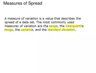
3.3 Measures of Spread
370 likes | 726 Vues
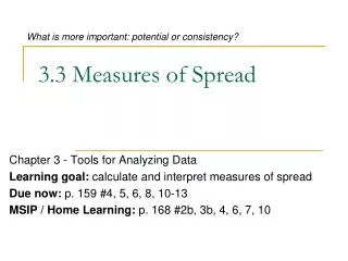
What is more important: potential or consistency?. 3.3 Measures of Spread. Chapter 3 - Tools for Analyzing Data Learning goal: calculate and interpret measures of spread Due now: p . 159 #4, 5, 6, 8, 10-13 MSIP / Home Learning: p. 168 #2b, 3b, 4, 6, 7, 10. What is spread?.

3.3 Measures of Spread
E N D
Presentation Transcript
What is more important: potential or consistency? 3.3 Measures of Spread Chapter 3 - Tools for Analyzing Data Learning goal: calculate and interpret measures of spread Due now: p. 159 #4, 5, 6, 8, 10-13 MSIP / Home Learning: p. 168 #2b, 3b, 4, 6, 7, 10
What is spread? • Measures of central tendency do not always tell you everything! • The histograms have identical mean and median, but the spread is different • Spread is how closely the values cluster around the middle value
Why worry about spread? • Less spread means you have greater confidence that values will fall within a particular range • Important for making predictions
Measures of Spread • We will also study 3 Measures of Spread: • Range • Interquartile Range (IQR) • Standard Deviation (Std.Dev.) • All 3 measure how spread out data is • Smaller value = less spread (more consistent) • Larger value = more spread (less consistent)
Measures of Spread • 1) Range = (max) – (min) • Indicates the size of the interval that contains 100% of the data • 2) Interquartile Range • IQR = Q3 – Q1, where • Q1 is the lower half median • Q3 is the upper half median • Indicates the size of the interval that contains the middle 50% of the data
Quartiles Example • 26 28 34 36 38 38 40 41 41 44 45 46 51 54 55 • Q2 = 41 Median • Q1 = 36 Lower half median • Q3 = 46 Upper half median • IQR = Q3 – Q1 • = 46 – 36 • = 10 • The middle 50% of the data is within 10 units • If a quartile occurs between 2 values, it is calculated as the average of the two values
A More Useful Measure of Spread • Range is very basic • Does not take clusters nor outliers into account • Interquartile Range is somewhat useful • Takes clusters into account • Visual in Box-and-Whisker Plot • Standard deviation is very useful • Average distance from the mean for all data points
Deviation • The mean of these numbers is 48 • Deviation = (data) – (mean) • The deviation for 24 is 24 - 48 = -24 • -24 • 12 24 36 48 60 72 84 • 36 • The deviation for 84 is 84 - 48 = 36
Calculating Standard Deviation 1. Find the mean (average) 2. Find the deviation for each data point data point – mean 3. Square the deviations (data point – mean)2 4. Average the squares of the deviations (this is called the variance) 5. Take the square root of the variance
Example of Standard Deviation • 26 28 34 36 • mean = (26 + 28 + 34 + 36) ÷ 4 = 31 • σ² = (26–31)² + (28-31)² + (34-31)² + (36-31)² 4 • σ² = 25 + 9 + 9 + 25 4 • σ² = 17 • σ = √17 = 4.1
Standard Deviation • σ² (lower case sigma squared) is used to represent variance • σ is used to represent standard deviation • σ is commonly used to measure the spread of data, with larger values of σ indicating greater spread • we are using a population standard deviation
Standard Deviation with Grouped Data • grouped mean = (2×2 + 3×6 + 4×6 + 5×2) / 16 = 3.5 • deviations: • 2: 2 – 3.5 = -1.5 • 3: 3 – 3.5 = -0.5 • 4: 4 – 3.5 = 0.5 • 5: 5 – 3.5 = 1.5 • σ² = 2(-1.5)² + 6(-0.5)² + 6(0.5)² + 2(1.5)² • 16 • σ² = 0.7499 • σ = √0.7499 = 0.9
Measure of Spread - Recap • Measures of Spread are numbers indicating how spread out data is • Smaller value for any measure of spread means data is more consistent • 1) Range = Max – Min • 2) Interquartile Range: IQR = Q3 – Q1, where • Q1 = first half median • Q3 = second half median • 3) Standard Deviation i. Find mean (average) ii. Find all deviations (data) – (mean) iii./iv. Square all and avgthem (this is variance or σ2) v. Take the square root to get std. dev. σ
MSIP / Home Learning • Read through the examples on pages 164-167 • Complete p. 168 #2b, 3b, 4, 6, 7, 10 • You are responsible for knowing how to do simple examples by hand (~6 pieces of data) • We will use technology (Fathom/Excel) to calculate larger examples • Have a look at your calculator and see if you have this feature (Σσn and Σσn-1)
“Think of how stupid the average person is, and realize half of them are stupider than that.” -George Carlin 3.4 Normal Distribution Chapter 3 – Tools for Analyzing Data Learning goal: Determine the % of data within intervals of a Normal Distribution Due now: p. 168 #2b, 3b, 4, 6, 7, 10 MSIP / Home Learning: p. 176 #1, 3b, 6, 8-10
Histograms • Histograms can be skewed... Right-skewed Left-skewed
Histograms • ... or symmetrical
Normal? • A normal distribution is a histogram that is symmetrical and has a bell shape • Used quite a bit in statistical analysis • Also called a Gaussian Distribution • Symmetrical with equal mean, median and mode that fall on the line of symmetry of the curve
A Real Example • the heights of 600 randomly chosen Canadian students from the “Census at School” data set • the data approximates a normal distribution
The 68-95-99.7% Rule • Area under curve is 1 (i.e. it represents 100% of the population surveyed) • Approx 68% of the data falls within 1 standard deviation of the mean • Approx 95% of the data falls within 2 standard deviations of the mean • Approx 99.7% of the data falls within 3 standard deviations of the mean • http://davidmlane.com/hyperstat/A25329.html
99.7% 95% 68% 34% 34% 0.15% 0.15% 13.5% 13.5% 2.35% 2.35% x - 3σ x - 2σ x - 1σ x x + 1σ x + 2σ x + 3σ Distribution of Data
Normal Distribution Notation • The notation above is used to describe the Normal distribution where x is the mean and σ² is the variance (square of the standard deviation) • e.g. X~N (70,82) describes a Normal distribution with mean 70 and standard deviation 8 (our class at midterm?)
An example • Suppose the time before burnout for an LED averages 120 months with a standard deviation of 10 months and is approximately Normally distributed. What is the length of time a user might expect an LED to last with: • a) 68% confidence? • b) 95% confidence? • So X~N(120,102)
An example cont’d • 68% of the data will be within 1 standard deviation of the mean • This will mean that 68% of the bulbs will be between 120–10 = 110 months and 120+10 = 130 months • So 68% of the bulbs will last 110 - 130 months • 95% of the data will be within 2 standard deviations of the mean • This will mean that 95% of the bulbs will be between 120 – 2×10 = 100 months and 120 + 2×10 = 140 months • So 95% of the bulbs will last 100 - 140 months
Example continued… • Suppose you wanted to know how long 99.7% of the bulbs will last? • This is the area covering 3 standard deviations on either side of the mean • This will mean that 99.7% of the bulbs will be between 120 – 3×10 months and 120 + 3×10 • So 99.7% of the bulbs will last 90-150 months • This assumes that all the bulbs are produced to the same standard
Example continued… 99.7% 95% µ represents the population mean What % of bulbs last between: µ - σ and µ + 2σ? 34 + 34 + 13.5 = 81.5% µ - 2σand µ? 13.5 + 34 = 47.5% 34% 34% 13.5% 13.5% 2.35% 2.35% 90 100 120 140 150 months months months months months
Percentage of data between two values • The area under any normal curve is 1 • The percent of data that lies between two values in a normal distribution is equivalent to the area under the normal curve between these values • See examples 2 and 3 on page 175
Why is the Normal distribution so important? • Many psychological and educational variables are distributed approximately normally: • height, reading ability, memory, IQ, etc. • Normal distributions are statistically easy to work with • All kinds of statistical tests are based on it • Lane (2003)
MSIP / Home Learning • Complete p. 176 #1, 3b, 6, 8-10 • http://onlinestatbook.com/
References • Lane, D. (2003). What's so important about the normal distribution? Retrieved October 5, 2004 from http://davidmlane.com/hyperstat/normal_distribution.html • Wikipedia (2004). Online Encyclopedia. Retrieved September 1, 2004 from http://en.wikipedia.org/wiki/Main_Page