Download
1 / 74
740 likes | 853 Vues
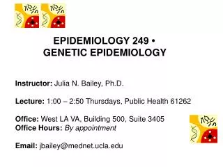
EPIDEMIOLOGY 249 • GENETIC EPIDEMIOLOGY. Instructor: Julia N. Bailey, Ph.D. Lecture: 1:00 – 2:50 Thursdays, Public Health 61262 Office: West LA VA, Building 500, Suite 3405 Office Hours: By appointment Email: jbailey@mednet.ucla.edu. Linkage:

E N D
EPIDEMIOLOGY 249 • GENETIC EPIDEMIOLOGY Instructor: Julia N. Bailey, Ph.D. Lecture: 1:00 – 2:50 Thursdays, Public Health 61262 Office: West LA VA, Building 500, Suite 3405 Office Hours:By appointment Email: jbailey@mednet.ucla.edu
Linkage: • Basic principles (revisiting Mendelian segregation) • Hardy Weinberg Equilibrium (HWE) • Inbreeding • Mendel segregation of traits - Linkage • genetic markers and maps • model-based linkage models • discrete trait linkage • pedigrees • LOD scores
Mendel’s First Law • Segregation ratio is ½ and parental transmissions are independent • A heterozygous parent (Aa) is equally likely to transmit either of the two alleles • What one parent transmits has no effect on the other parent
Question? If a trait is recessive does that mean that one in four people will have that trait? Hint - we have to think in terms of allele frequencies and genotype frequencies in the population.
Allele frequency • Definition: • The probability that a gene selected at random will be of a specific type • Frequency of ‘A’ is p • Frequency of ‘a’ is q
Genotype Frequencies Three types of genotypes – AA, Aa, AA p= f(AA) + ½ f(Aa) q= f(aa) + ½ f(Aa) f(AA)+f(Aa)+f(aa)=1=p+q
Calculating p&q by gene counting Population has the following individuals: AA, Aa, AA, Aa, aa, AA, AA, AA, Aa, Aa (10 individuals = 20 alleles) f(AA)=p=(2+1+2+1+0+2+2+2+1+1)/20 =14/20=0.7 f(aa) = q = (0+1+0+1+2+0+0+0+1+1)/20 =6/20=0.3 (q=1-p)
Godfrey Harold Hardy (1877 – 1947) was a prominent English mathematician who left his mark in the field of population genetics in addition to mathematics. He played cricket with the geneticist Reginald Punnett who introduced the problem to him. Dr Wilhelm Weinberg (1862 — 1937) was a German physician who in 1908 independently formulated the Hardy-Weinberg principle. The Hardy–Weinberg principle states that both allele and genotype frequencies in a population remain constant or are in equilibrium from generation to generation unless specific disturbing influences are introduced.
Hardy-Weinberg Equilibrium • Predicts genotype frequencies from allele frequencies AA = p2 Aa = 2pq aa = q2 • Populations will be in HWE in one generation unless specific disrupting influences are introduced.
Test of H-W equilibrium • Simple chi-square test (goodness of fit) • Compare observed to expected allele frequencies
Calculating HWE AA, Aa, AA, Aa, aa, AA, AA, AA, Aa, Aa p=0.7, q=0.3 2 = 0.01, p=0.99
Causes of Deviations from Hardy-Weinberg Genotype Frequencies • Assortative (non-random) mating • Ethnic/racial/regional groups, endogamy • Inbreeding or consanguineous mating • Changing allele frequencies • Genetic drift (small populations only) • Selection, mortality, mutation, migration • Genotyping error • Tends to increase homozygosity
Effect of Inbreeding • Predicted genotype frequencies: PAA = p2 (1-f) + pf PAa = 2pq(1-f) Paa = q2(1-f)+qf f is the ‘inbreeding coefficient’
Bennett et al. (2002) • Consanguineous matings increase rates of recessive genetic disease, but most such diseases are rare such that a large relative risk may still imply a small absolute risk • Current laws prohibiting first-cousin marriages are overly restrictive
King Charles II of Spain, the product of generations of inbreeding by the Hapsburg family. This is a man whose face and chin were so distorted by the "Hapsburg Lip" that he could not eat without assistance. He also had cognitive issues.
Mendel’s peas again… Going from segregation to linkage…
Dihybrid Cross • Study transmission of two traits simultaneously • Start with plants that are purebred for two traits • e.g., round yellow seeds and wrinkled green seeds • Yellow is dominant over green • Round is dominant over wrinkled • Cross these to produce round yellow ‘dihybrids’ • Cross the dihybrid plants to produce a variety of combinations of traits F0 F1 F2
Takes 2 generations to see results AA X aa F0 X F0 produces F1 (Filial 1) Aa X Aa F1 X F1 produces F2 AA, Aa, aa (1/4, ½, ¼)
Mendel’s Second Law • Independent Assortment • Segregations for two traits are independent • Mendel was wrong on this one! • He studied pairs of traits that showed independence • e.g., color and shape of seeds • Some traits that he studied separately would not have shown independence if he had studied them jointly because THEY WERE LINKED ON THE CHROMOSOME
Thomas Hunt Morgan • amount of crossing over between linked genes differs led to the idea that crossover frequency might indicate the distance separating genes on the chromosome.
Alfred Sturtevant (1913). J. Exper. Zool. • showed genes have a "linear arrangement" – ordered • developed recombination fraction • Centimorgan (cM) is defined as the distance between genes (DNA) for which one product of meiosis in 100 is recombinant. • A recombinant frequency (RF) of 1 % is equivalent to 1 genetic map unit. (mu)
Recombination Fraction • The proportion of meioses that produced a recombinant between the two loci will always range between 0 and 0.5. This proportion is called the recombination fraction and is usually denoted (theta).
T U t u T t U u Here, there will be few recombinaints, and will be near zero. Here, there will be many recombinants and will be greater than zero. The number of recombinants is directly related to the distance between the loci. is a measure of distance
Exercise: Estimate # recombinants (# recombinants+ # non-recombinants) = 1/(1+5) = 0.17
Genetic Map Physical Map Recombination fraction base pairs (bp, or Mb) • As a very rough rule of thumb, 1 cM on a chromosome encompasses 1 megabase (1 Mb = 100 bp) of DNA. • this relationship is only approximate. • Genetic maps of human females average 90% longer than the same maps in males, their chromosomes contain the same number of base pairs. So their physical maps are identical.
Linkage Analyses (Finally!) Two point Linkage analyses Disease & Marker Marker & Marker (that’s how they made the map).
Ex Calculating by HandABO Blood Group • Blood types: A, B, AB and O • Alleles: IA, IB and i • Genotypes: • A is either IA i or IA IA • B is either IB i or IB IB • AB is always IA IB • O is always i i
Exercise:Computing by Hand # Recombinants = 2 # Non Recombinants = ?
Problems • Assumed phase (need to consider both) • Assumed complete dominant penetrance • Assumed complete genotype data (no missing data). • Direct method may be biased.
Maximum likelihood estimator of recombination • Extracts all linkage information (e.g. phase)
LOD scores • Measure evidence for linkage • Logarithm of the Odds (odds for linkage vs odds against linkage) • z is used directly as the indicator of significance. • z greater than 3.0 (3.3) is taken as significant evidence for linkage. • z less than –2.0 is taken as significant evidence against linkage.
Z()=log10[L]- log10[L(=0.5)] • Various are estimated – usually at 0, 0.1, 0.2, 0.3, 0.4 • Lodscores are computed for each family • Lodscores of multiple families are just summed across families. • Maximum Lods are the highest lod obtained (maximizing )
Benefits • Likelihood of the pedigree, given specific parameters • Distance between disease & marker is • Disease is modeled with specific inheritance patterns, e.g. dominant/recessive/additive, gene frequency, autosomal or X linked • Can incorporate parameters for missing data,