Inverse reinforcement learning(IRL) a pproach to modeling pastoralist movements

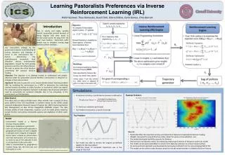
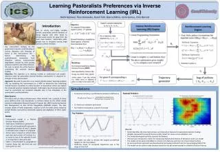
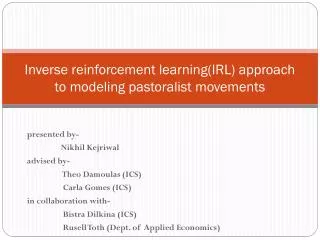
1. Inverse reinforcement learning(IRL) approach to modeling pastoralist movements presented by- Nikhil Kejriwal advised by- Theo Damoulas (ICS) Carla Gomes (ICS) in collaboration with- BistraDilkina (ICS) RusellToth (Dept. of Applied Economics)

2. Outline • Background • Reinforcement Learning • Inverse Reinforcement Learning (IRL) • Pastoral Problem • Model • Results

3. Pastoralists of Africa • Survey was collected by the USAID Global Livestock Collaborative Research Support Program (GL CRSP) under PARIMA project by Prof C. B. Barrett. • The project focuses on six locations in Northern Kenya and Southern Ethiopia • We wish to explain the movement over time and space of animal herders • The movement of herders is due to highly variable rainfall: in between winters and summers, there are dry seasons, with virtually no precipitation. Herds migrate to remote water points. • Pastoralists can suffer greatly by droughts, by losing large portions of their herds • We are interested in the herders spatiotemporal movement problem to understand the incentives on which they base their decisions. This can help form policies (control of grazing, drilling water points)

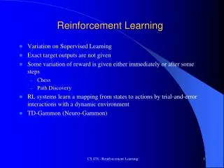
4. Reinforcement Learning • Common form of learning among animals. • Agent interacts with an environment (takes an action) • Transitions into a new state • Gets a positive or negative reward

5. Reinforcement Learning Environment Model (MDP) • Goal: Pick actions over time so as to maximize the expected score: E[R(s0) + R(s1) + … + R(sT)] • Solution: policy  which specifies an action for each possible state Reinforcement Learning Optimal policy p Reward Function R (s)

6. Inverse Reinforcement Learning Environment Model (MDP) Inverse Reinforcement Learning (IRL) Optimal policy p Reward Function R (s) R that explains expert trajectories Expert Trajectories s0, a0, s1, a1 , s2, a2 …

7. Reinforcement Learning • MDP is represented as a tuple (S, A, {Psa}, ,R) R is bounded by Rmax • Value function for policy : • Q-function:

8. Bellman Equation: • Bellman Optimality:

9. Inverse Reinforcement Learning • Linear approximationof reward function some using basis functions • Let be value function of policy , when reward R = • For computing R thatmakes optimal

10. Inverse Reinforcement Learning • Expert policy is only accessible through a set of sampled trajectories • For a trajectory state sequence (s0, s1, s2….): • Considering just the ith basis function • Note that this is the sum of discounted features along a trajectory • Estimated value will be :

11. Inverse Reinforcement Learning • Assume we have some set of policies • Linear Programming formulation • The above optimization gives a new reward R, we then compute based on R, and add it to the set of policies • reiterate (Andrew Ng & Struat Russell, 2000)

12. Apprenticeship learning to recover R • Find Rs.t. R is consistent with the teacher’s policy * being optimal. • Find Rs.t.: • Find t,w: (Pieter Abbeel & Andrew Ng, 2004)

13. Pastoral Problem • We have data describing: • Household information from 5 villages • Lat, Long information of all water points(311) and villages • All the water points visited over the last quarter by a sub herd • Time spent at each water point • Estimated capacity of the water point • Vegetation information around the water points • Herd sizes and types • We have been able to generate around 1750 expert trajectories described over a period of 3 months (~90 days)

14. All water points

15. All trajectories

16. Sample trajectories

17. State Space • Model: • State is uniquely identified by geographical location (long, lat) and the herd size. • S = (Long, Lat, Herd) • A = (Stay, Move to adjacent cell on the grid) • 2nd option for Model • S = (wp1, wp2, Herd) • A = (stay at same edge, move to another edge) • Larger State space

18. Modeling Reward • Linear Model • R(s) = th * [veg(long,lat), cap(long,lat), herd_size, is_village(long,lat), … interaction_terms]; • Normalized values of veg, cap, herd_size • RBF Model • 30 basis functions fi(s) • R(s) = sum (thi * fi(s)) i = 1,2,…30 • s = veg(long,lat), cap(long,lat), herd_size, is_village(long,lat)

19. Toy Problem • Used exactly the same model • Pre-defined the weights th, got a reward function R(s) • Used a synthetic generator to generate expert policy and trajectories • Ran IRL to generate a reward function • Compared computed reward with known reward

20. Toy Problem

21. Linear Reward Model- recovered from pastoral trajectories

23. RBFReward Model- recovered from pastoral trajectories

24. Currently working on … • Including time as another dimension in the state space • Specifying a performance metric for recovered reward function • Cross validation • Specifying a better/novel reward function

25. Thank You • Questions / Comments

27. Weights computed by running IRL on the actual problem

29. Algorithm • For t = 1,2,… • Inverse RL step: • Estimate expert’s reward function R(s)= wT(s) such that under R(s) the expert performs better than all previously found policies {i}. • RL step: • Compute optimal policy t for • the estimated reward w. Courtesy of Pieter Abbeel

30. Algorithm: IRL step • Maximize, w:||w||2≤ 1 • s.t. Vw(E)  Vw(i) +  i=1,…,t-1 •  = margin of expert’s performance over the performance of previously found policies. • Vw() = E[t t R(st)|] = E[t t wT(st)|] • = wTE[t t (st)|] • = wT () • () = E[t t (st)|] are the “feature expectations” Courtesy of Pieter Abbeel

31. Feature Expectation Closeness and Performance • If we can find a policy  such that • ||(E) - ()||2 , • then for any underlying reward R*(s) =w*T(s), • we have that • |Vw*(E) - Vw*()| = |w*T (E) - w*T ()| •  ||w*||2 ||(E) - ()||2 • . Courtesy of Pieter Abbeel

32. Algorithm • For i = 1, 2, … • Inverse RL step: • RL step: (= constraint generation) Compute optimal policy i for the estimated reward Rw.