Reinforcement Learning
Reinforcement Learning. Agenda. Online learning Reinforcement learning Model-free vs. model-based Passive vs. active learning Exploration-exploitation tradeoff. Incremental (“Online”) Function Learning. Data is streaming into learner x 1 ,y 1 , …, x n ,y n y i = f(x i )

Reinforcement Learning
E N D
Presentation Transcript
Agenda • Online learning • Reinforcement learning • Model-free vs. model-based • Passive vs. active learning • Exploration-exploitation tradeoff
Incremental (“Online”) Function Learning • Data is streaming into learnerx1,y1, …, xn,ynyi = f(xi) • Observes xn+1 and must make prediction for next time step yn+1 • “Batch” approach: • Store all data at step n • Use your learner of choice on all data up to time n, predict for time n+1 • Can we do this using less memory?
Example: Mean Estimation • yi = q + error term (no x’s) • Current estimate qn = 1/n Si=1…nyi • qn+1 = 1/(n+1) Si=1…n+1yi = 1/(n+1) (yn+1 + Si=1…nyi) = 1/(n+1) (yn+1 + n qn)= qn+ 1/(n+1) (yn+1- qn) q5
Example: Mean Estimation • yi = q + error term (no x’s) • Current estimate qt = 1/n Si=1…nyi • qn+1 = 1/(n+1) Si=1…n+1yi = 1/(n+1) (yn+1 + Si=1…nyi) = 1/(n+1) (yn+1 + n qn) = qn+ 1/(n+1) (yn+1 - qn) y6 q5
Example: Mean Estimation • yi = q + error term (no x’s) • Current estimate qt = 1/n Si=1…nyi • qn+1 = 1/(n+1) Si=1…n+1yi = 1/(n+1) (yn+1 + Si=1…nyi) = 1/(n+1) (yn+1 + n qn) = qn+ 1/(n+1) (yn+1 - qn) q5 q6 = 5/6 q5 + 1/6 y6
Example: Mean Estimation • qn+1 = qn + 1/(n+1) (yn+1 - qn) • Only need to store n, qn q5 q6 = 5/6 q6 + 1/6 y6
Learning Rates • In fact, qn+1 = qn + an (yn+1 - qn) converges to the mean for any an such that: • an 0 as n • San • San2C < • O(1/n) does the trick • If an is close to 1, then the estimate shifts strongly to recent data; close to 0, and the old estimate is preserved
Reinforcement Learning • RL problem: given only observations of actions, states, and rewards, learn a (near) optimal policy • No prior knowledge of transition or reward models • We consider: fully-observable, episodic environment, finite state space, uncertainty in action (MDP)
What to Learn? Model free Model based Less online deliberation More online deliberation Action-utilityfunction Q(s,a) Utilityfunction U Model of R and T Policy p Learn: argmaxaSsP(s’|s,a)U(s’) Solve MDP argmaxaQ(s,a) Online: p(s) Method: Learning from demonstration Q-learning, SARSA Direct utility estimation, TD-learning Adaptive dynamic programming Simpler execution Fewer examples needed to learn?
First steps: Passive RL • Observe execution trials of an agent that acts according to some unobserved policy p • Problem: estimatethe utility function Up • [Recall Up(s) = E[StgtR(St)] where St is the random variable denoting the distribution of states at time t]
0 0.81 0.87 0 0 0.92 +1 +1 3 3 0.76 0 0.66 0 -1 -1 2 2 0.71 0 0 0.66 0 0.61 0.39 0 1 1 1 1 2 2 3 3 4 4 Direct Utility Estimation • Observe trials t(i)=(s0(i),a1(i),s1(i),r1(i),…,ati(i),sti(i),rti(i)) for i=1,…,n • For each state sS: • Find all trials t(i) that pass through s • Compute subsequent utility Ut(i)(s)=St=k to tigt-k rt(i) • Set Up(s) to the average observed utility
0.81 0 0 0.87 0.92 0 +1 +1 3 3 0 0.76 0 0.66 -1 -1 2 2 0 0.71 0 0.66 0 0.61 0 0.39 1 1 1 1 2 2 3 3 4 4 Online Implementation • Store counts N[s] and estimated utilities Up(s) • After a trial t, for each state s in the trial: • Set N[s] N[s]+1 • Adjust utility Up(s) Up(s)+a(N[s])(Ut(s)-Up(s)) • Simply supervised learning on trials • Slow learning, because Bellman equation is not used to pass knowledge between adjacent states
0 0 0 +1 3 0 0 -1 2 0 0 0 0 1 1 2 3 4 Temporal Difference Learning • Store counts N[s] and estimated utilities Up(s) • For each observed transition (s,r,a,s’): • Set N[s] N[s]+1 • Adjust utility Up(s) Up(s)+a(N[s])(r+gUp(s’)-Up(s))
0 0 0 +1 3 0 0 -1 2 0 0 0 0 1 1 2 3 4 Temporal Difference Learning • Store counts N[s] and estimated utilities Up(s) • For each observed transition (s,r,a,s’): • Set N[s] N[s]+1 • Adjust utility Up(s) Up(s)+a(N[s])(r+gUp(s’)-Up(s))
0 0 0 +1 3 0 0 -1 2 -0.02 0 0 0 1 1 2 3 4 Temporal Difference Learning With learning rate a=0.5 • Store counts N[s] and estimated utilities Up(s) • For each observed transition (s,r,a,s’): • Set N[s] N[s]+1 • Adjust utility Up(s) Up(s)+a(N[s])(r+gUp(s’)-Up(s))
-0.02 -0.02 0 +1 3 -0.02 0 -1 2 -0.02 0 0 0 1 1 2 3 4 Temporal Difference Learning With learning rate a=0.5 • Store counts N[s] and estimated utilities Up(s) • For each observed transition (s,r,a,s’): • Set N[s] N[s]+1 • Adjust utility Up(s) Up(s)+a(N[s])(r+gUp(s’)-Up(s))
-0.02 -0.02 0.48 +1 3 -0.02 0 -1 2 -0.02 0 0 0 1 1 2 3 4 Temporal Difference Learning With learning rate a=0.5 • Store counts N[s] and estimated utilities Up(s) • For each observed transition (s,r,a,s’): • Set N[s] N[s]+1 • Adjust utility Up(s) Up(s)+a(N[s])(r+gUp(s’)-Up(s))
-0.04 0.21 0.72 +1 3 -0.04 0 -1 2 -0.04 0 0 0 1 1 2 3 4 Temporal Difference Learning With learning rate a=0.5 • Store counts N[s] and estimated utilities Up(s) • For each observed transition (s,r,a,s’): • Set N[s] N[s]+1 • Adjust utility Up(s) Up(s)+a(N[s])(r+gUp(s’)-Up(s))
0.07 0.44 0.84 +1 3 -0.06 0 -1 2 -0.06 0 0 0 1 1 2 3 4 Temporal Difference Learning With learning rate a=0.5 • Store counts N[s] and estimated utilities Up(s) • For each observed transition (s,r,a,s’): • Set N[s] N[s]+1 • Adjust utility Up(s) Up(s)+a(N[s])(r+gUp(s’)-Up(s))
0.23 0.62 0.42 +1 3 -0.03 0 -1 2 -0.08 0 0 0 1 1 2 3 4 Temporal Difference Learning With learning rate a=0.5 • Store counts N[s] and estimated utilities Up(s) • For each observed transition (s,r,a,s’): • Set N[s] N[s]+1 • Adjust utility Up(s) Up(s)+a(N[s])(r+gUp(s’)-Up(s))
0.23 0.62 0.42 +1 3 -0.03 0.19 -1 2 -0.08 0 0 0 1 1 2 3 4 Temporal Difference Learning With learning rate a=0.5 • Store counts N[s] and estimated utilities Up(s) • For each observed transition (s,r,a,s’): • Set N[s] N[s]+1 • Adjust utility Up(s) Up(s)+a(N[s])(r+gUp(s’)-Up(s))
0.23 0.62 0.69 +1 3 -0.03 0.19 -1 2 -0.08 0 0 0 1 1 2 3 4 Temporal Difference Learning With learning rate a=0.5 • Store counts N[s] and estimated utilities Up(s) • For each observed transition (s,r,a,s’): • Set N[s] N[s]+1 • Adjust utility Up(s) Up(s)+a(N[s])(r+gUp(s’)-Up(s)) • For any s, distribution of s’ approaches P(s’|s,p(s)) • Uses relationships between adjacent states to adjust utilities toward equilibrium • Unlike direct estimation, learns before trial is terminated
0 0 0 +1 +1 3 3 0 0 -1 -1 2 2 0 0 0 ? 0 1 1 1 1 2 2 3 3 4 4 “Offline” interpretation of TD Learning • Observe trials t(i)=(s0(i),a1(i),s1(i),r1(i),…,ati(i),sti(i),rti(i)) for i=1,…,n • For each state sS: • Find all trials t(i) that pass through s • Extract local history at (s,r(i),a(i),s’(i)) for each trial • Set up constraint Up(s) = r(i) + gUp(s’(i)) • Solve all constraints in least squares fashion using stochastic gradient descent • [Recall linear system in policy iteration: u = r+Tpu]
-.04 0 0 -.04 -.04 0 +1 +1 3 0 -.04 0 -.04 -1 -1 2 0 -.04 0 -.04 0 -.04 ? 0 ? 1 1 2 3 4 Adaptive Dynamic Programming R(s) P(s’|s,a) • Store counts N[s],N[s,a],N[s,a,s’],estimated rewards R(s), and transition model P(s’|s,a) • For each observed transition (s,r,a,s’): • Set N[s] N[s]+1, N[s,a] N[s,a]+1, N[s,a,s’] N[s,a,s’]+1 • Adjust reward R(s) R(s)+a(N[s])(r-R(s)) • Set P(s’|s,a) = N[s,a,s’]/N[s,a] • Solve policy evaluation using P, R, p • Faster learning than TD, because Bellman equation is exploited across all states • Modified policy evaluation algorithms make updates faster than solving linear system (O(n3))
Active RL • Rather than assume a policy is given, can we use the learned utilities to pick good actions? • At each state s, the agent must learn outcomes for all actions, not just the action p(s)
Greedy RL • Maintain current estimates Up(s) • Idea: At state s, take action a that maximizess’ P(s’|s,a) Up(s’) • Very seldom works well! Why?
Exploration vs. Exploitation • Greedy strategy purely exploits its current knowledge • The quality of this knowledge improves only for those states that the agent observes often • A good learner must perform exploration in order to improve its knowledge about states that are not often observed • But pure exploration is useless (and costly) if it is never exploited
Optimistic Exploration Strategy • Behave initially as if there were wonderful rewards R+ scattered all over the place • Define a modified optimistic Bellman updateU+(s) R(s)+gmaxaf(SsP(s’|s,a)U+(s’) , N[s,a]) Truncated exploration function: f(u,n) = R+if n < Ne u otherwise [Here the agent will try each action in each state at least Ne times.]
Complexity • Truncated: at least Ne·|S|·|A| steps are needed in order to explore every action in every state • Some costly explorations might not be necessary, or the reward from far-off explorations may be highly discounted • Convergence to optimal policy guaranteed only if each action is tried in each state an infinite number of times! • This works with ADP… But how to perform action selection in TD? • Must also learn the transition model P(s’|s,a)
Q-Values • Learning U is not enough for action selection because a transition model is needed • Solution: learn Q-values: Q(s,a) is the utility of choosing action a in state s • Shift Bellman equation • U(s) = maxa Q(s,a) • Q(s,a) = R(s) + gSsP(s’|s,a)maxa’ Q(s’,a’) • So far, everything is the same… but what about the learning rule?
Q-learning Update • Recall TD: • Update: U(s) U(s)+a(N[s])(r+gU(s’)-U(s)) • Select action: a argmaxaf(Ss P(s’|s,a)U(s’) , N[s,a]) • Q-Learning: • Update: Q(s,a) Q(s,a)+a(N[s,a])(r+gmaxa’Q(s’,a’)-Q(s,a)) • Select action: a argmaxaf(Q(s,a) , N[s,a]) • Key difference: average over P(s’|s,a) is “baked in” to the Q function • Q-learning is therefore a model-free active learner
More Issues in RL • Model-free vs. model-based • Model-based techniques are typically better at incorporating prior knowledge • Generalization • Value function approximation • Policy search methods
Large Scale Applications • Game playing • TD-Gammon: neural network representation of Q-functions, trained via self-play • Robot control
Recap • Online learning: learn incrementally with low memory overhead • Key differences between RL methods: what to learn? • Temporal differencing: learn U through incremental updates. Cheap, somewhat slow learning. • Adaptive DP: learn P and R, derive U through policy evaluation. Fast learning but computationally expensive. • Q-learning: learn state-action function Q(s,a), allows model-free action selection • Action selection requires trading off exploration vs. exploitation • Infinite exploration needed to guarantee that the optimal policy is found!
Incremental Least Squares • Recall Least Squares estimateq = (ATA)-1 AT b • Where A is matrix of x(i)’s, b is vector of y(i)’s (laid out in rows) NxM Nx1 x(1) y(1) x(2) y(2) A = b = … … x(N) y(N)
Delta Rule for Linear Least Squares • Delta rule (Widrow-Hoff rule): stochastic gradient descentq(t+1) = q(t)+ax (y-q(t)Tx) • O(n) time and space
Incremental Least Squares • Let A(t), b(t)be A matrix,b vector up to time tq(t) = (A(t)TA(t))-1 A(t)T b(t) (T+1)xM (t+1)x1 A(t+1) = A(t) b(t+1) = b(t) x(t+1) y(t+1)
Incremental Least Squares • Let A(t), b(t)be A matrix, b vector up to time tq(t+1) = (A(t+1)TA(t+1))-1 A(t+1)T b(t+1) • A(t+1)T b(t+1) =A(t)T b(t) + y(t+1)x(t+1) (T+1)xM (t+1)x1 A(t+1) = A(t) b(t+1) = b(t) x(t+1) y(t+1)
Incremental Least Squares • Let A(t), b(t)be A matrix, b vector up to time tq(t+1) = (A(t+1)TA(t+1))-1 A(t+1)T b(t+1) • A(t+1)T b(t+1) =A(t)T b(t) + y(t+1)x(t+1) • A(t+1)TA(t+1) = A(t)TA(t) + x(t+1)x(t+1)T (T+1)xM (t+1)x1 A(t+1) = A(t) b(t+1) = b(t) x(t+1) y(t+1)
Incremental Least Squares • Let A(t), b(t)be A matrix, b vector up to time tq(t+1) = (A(t+1)TA(t+1))-1 A(t+1)T b(t+1) • A(t+1)T b(t+1) =A(t)T b(t) + y(t+1)x(t+1) • A(t+1)TA(t+1) = A(t)TA(t) + x(t+1)x(t+1)T (T+1)xM (t+1)x1 A(t+1) = A(t) b(t+1) = b(t) x(t+1) y(t+1)
Incremental Least Squares • Let A(t), b(t)be A matrix, b vector up to time tq(t+1) = (A(t+1)TA(t+1))-1 A(t+1)T b(t+1) • A(t+1)T b(t+1) =A(t)T b(t) + y(t+1)x(t+1) • A(t+1)TA(t+1) = A(t)TA(t) + x(t+1)x(t+1)T • Sherman-Morrison Update • (Y + xxT)-1 = Y-1 - Y-1xxT Y-1 / (1 – xT Y-1 x)
Incremental Least Squares • Putting it all together • Store p(t) = A(t)Tb(t) Q(t) = (A(t)TA(t))-1 • Update p(t+1) = p(t) + y x Q(t+1) = Q(t) - Q(t)xxT Q(t) / (1 – xT Q(t) x)q(t+1) = Q(t+1)p(t+1) • O(M2) time and space instead of O(M3+MN) time and O(MN) space for OLS • True least squares estimator for any t, (delta rule works only for large t)

