Exploring Reinforcement Learning: Passive vs Active Approaches
Learn about reinforcement learning, passive vs active learning, model-based vs model-free approaches, and techniques like Direct Estimation, Adaptive Dynamic Programming, and Temporal Difference Learning.

Exploring Reinforcement Learning: Passive vs Active Approaches
E N D
Presentation Transcript
So far …. • Given an MDP model we know how to find optimal policies • Value Iteration or Policy Iteration • Later in class we will show how to find policies given just a simulator of an MDP • But what if we don’t have any form of model • Like when we were babies . . . • Like in many real-world applications • All we can do is wander around the world observing what happens, getting rewarded and punished • Enters reinforcement learning 2
Reinforcement Learning • No knowledge of environment • Can only act in the world and observe states and reward • Many factors make RL difficult: • Actions have non-deterministic effects • Which are initially unknown • Rewards / punishmentsare infrequent • Often at the end of long sequences of actions • How do we determine what action(s) were really responsible for reward or punishment? (credit assignment) • World is large and complex • Nevertheless learner must decidewhat actions to take • We will assume the world behaves as an MDP 3
Passive vs. Active learning • Passive learning • The agent has a fixed policy and tries to learn the utilities of states by observing the world go by • Analogous to policy evaluation • Often serves as a component of active learning algorithms • Often inspires active learning algorithms • Active learning • The agent attempts to find an optimal (or at least good) policy by acting in the world • Analogous to solving the underlying MDP 4
Model-Based vs. Model-Free RL • Model based approach to RL: • learn the MDP model, or an approximation of it • use it for policy evaluation or to find the optimal policy • Model free approach to RL: • derive the optimal policy without explicitly learning the model • useful when model is difficult to represent and/or learn • We will consider both types of approaches 5
Passive RL in a known environment Passive Learner: A passive learner simply watches the world going by, and tries to learn the utility of being in various states. Another way to think of a passive learner is as an agent with a fixed policy trying to determine its benefits. Utilities can be learned using 3 approaches • LMS (least mean squares) • ADP (adaptive dynamic programming) • TD (temporal difference learning)
Objective: Value Function • Agent is provided: Mi j=a model given the probability of reaching from state i to state j (each state transitions to neighbouring states with equal probability). 7
Estimate U(s) Follow the policy for many epochs giving training sequences. Assume that after entering +1 or -1 state the agent enters zero reward terminal state So we don’t bother showing those transitions Passive RL (1,1)(1,2)(1,3)(1,2)(1,3)(2,3)(3,3) (3,4)+1 (1,1)(1,2)(1,3)(2,3)(3,3)(3,2)(3,3)(3,4) +1 (1,1)(2,1)(3,1)(3,2)(4,2) -1 8
Approach 1: Direct Estimation = LMS • Direct estimation (model free) • Estimate U(s) as average total reward of epochs containing s (calculating from s to end of epoch) • Reward to go of a state s the sum of the (discounted) rewards from that state until a terminal state is reached • Key: use observed reward to go of the state as the direct evidence of the actual expected utility of that state. • What is the reward to go for state (1,2)? • Averaging the reward to go samples will converge to true value at state 9
Direct Estimation • Converge very slowly to correct utilities values (requires a lot of sequences) • Doesn’t exploit Bellman constraints on policy values How can we incorporate constraints? 10
Approach 2: Adaptive Dynamic Programming (ADP) • ADP is a model based approach • Follow the policy for awhile • Learn reward function for each state • Compute utility of policy, using value determination • The agent is passive, hence no maximization over actions. 11
Approach 3: Temporal Difference Learning (TD) • Can we avoid the computational expense of full DP policy evaluation? • Temporal Difference Learning (model free) • Do local updates of utility/value function on a per-action basis • Don’t try to estimate entire transition function! • For each transition from i to j, we perform the following update: • Intuitively moves us closer to satisfying Bellman constraint • is a learning rate parameter. It can be adaptive for good convergence. 12
The TD learning curve • Tradeoff: requires more training experience (epochs) than ADP but much less computation per epoch • Choice depends on relative cost of experience vs. computation 13
Passive RL: Comparisons • Direct Estimation (model free) • Simple to implement • Each update is fast • Does not exploit Bellman constraints • Converges slowly • Adaptive Dynamic Programming (model based) • Harder to implement • Each update is a full policy evaluation (expensive) • Fully exploits Bellman constraints • Fast convergence (in terms of updates) • Temporal Difference Learning (model free) • Update speed and implementation similar to direct estimation • Partially exploits Bellman constraints---adjusts state to ‘agree’ with observed successor • Not all possible successors • Convergence in between direct estimation and ADP 14
Between ADP and TD Moving TD toward ADP At each step update based on observed transition and “imagined” transitions Imagined transition are generated using estimated model The more imagined transitions the more like ADP Making estimate more consistent with next state distribution 15
Passive RL in an unknown environment • Least Mean Square(LMS) approach and Temporal-Difference(TD) approach operate unchanged in an initially unknown environment. • Adaptive Dynamic Programming(ADP) approach adds a step that updates an estimated model of the environment.
ADP approach • The environment model is learned by direct observation of transitions. • The environment model M can be updated by keeping track of the percentage of times each state transitions to each of its neighbors. • There are efficient approximate versions of the algorithm.
Active Reinforcement Learning • So far, we’ve assumed agent hasapolicy • We just learned how good it is • Now, suppose agent must learn a good policy (ideally optimal) • While acting in uncertain world 18
Naïve Approach • Act Randomly for a (long) time • Or systematically explore all possible actions • Learn • Transition function • Reward function • Use value iteration, policy iteration, … • Follow resulting policy thereafter. Will this work? 19
Revision of Naïve Approach Start with initial utility/value function and initial model Take greedy action according to value function|(this requires using our estimated model to do “lookahead”) Update estimated model Perform step of ADP ;; update value function Goto 2 This is just ADP but we follow the greedy policy suggested by current value estimate Will it work? No. Can get stuck in local minima. 20
Exploration versus Exploitation • Two reasons to take an action in RL • Exploitation: To try to get reward. We exploit our current knowledge to get a payoff. • Exploration: Get more information about the world. How do we know if there is not a pot of gold around the corner. • To explore we typically need to take actions that do not seem best according to our current model. • Managing the trade-off between exploration and exploitation is a critical issue in RL • Basic intuition behind most approaches: • Explore more when knowledge is weak • Exploit more as we gain knowledge 21
ADP-based RL • Start with initial utility/value function • Take action according to an explore/exploit policy(explores more early on and gradually becomes greedy) • Update estimated model • Perform step of ADP • Goto 2 This is just ADP but we follow the explore/exploit policy Will this work? Depends on the explore/exploit policy. Any ideas? 22
Explore/Exploit Policies • Greedy action is action maximizing estimated Q-value • where V is current value function estimate, and R, T are current estimates of model • Q(s,a) is the expected value of taking action a in state s and then getting the estimated value V(s’) of the next state s’ • Want an exploration policy that is greedy in the limit of infinite exploration (GLIE) • Guarantees convergence • Solution 1 • On time step t select random action with probability p(t) and greedy action with probability 1-p(t) • p(t) = 1/t will lead to convergence, but is slow 23
Explore/Exploit Policies • Greedy action is action maximizing estimated Q-value • where V is current value function estimate, and R, T are current estimates of model • Solution 2: Boltzmann Exploration • Select action a with probability, • T is the temperature. Large T means that each action has about the same probability. Small T leads to more greedy behavior. • Typically start with large T and decrease with time 24
The Impact of Temperature • Suppose we have two actions and that Q(s,a1) = 1, Q(s,a2) = 2 • T=10 gives Pr(a1 | s) = 0.48, Pr(a2 | s) = 0.52 • Almost equal probability, so will explore • T= 1 gives Pr(a1 | s) = 0.27, Pr(a2 | s) = 0.73 • Probabilities more skewed, so explore a1 less • T = 0.25 gives Pr(a1 | s) = 0.02, Pr(a2 | s) = 0.98 • Almost always exploit a2 25
Alternative Approach:Optimistic Exploration • Start with initial utility/value function • Take greedy action • Update estimated model • Perform step of optimistic ADP(uses optimistic variant of value iteration)(inflates value of actions leading to unexplored regions) • Goto 2 Basically act as if all “unexplored” state-action pair are maximally rewarding. 26
Optimistic Exploration • Recall that value iteration iteratively performs the following update at all states: • Adjust update to make actions that lead to unexplored regions look good • Implement variant of VI that assigns the highest possible value Vmax to any state-action pair that has not been explored enough • Maximum value is when we get maximum reward forever • What do we mean by “explored enough”? • N(s,a) > Ne, where N(s,a) is number of times action a has been tried in state s and Ne is a user selected parameter 27
Optimistic Exploration • Optimistic value iteration computes an optimistic value function V+ using updates • The agent will behave initially as if there were wonderful rewards scattered all over around– optimistic . • But after actions are tried enough times we will perform standard “non-optimistic” value iteration • Some recent theoretical results show how to set Ne is to arrive at provably optimal learning (with high probability) in polynomial time (the RMAX algorithm) 28
TD-based Active RL • Start with initial utility/value function • Take action according to an explore/exploit policy(should converge to greedy policy, i.e. GLIE) • Update estimated model • Perform TD updateV(s) is new estimate of optimal value function at state s. • Goto 2 Just like TD for passive RL, but we follow explore/exploit policy Given the usual assumptions about learning rate and GLIE, TD will converge to an optimal value function! 29
TD-based Active RL • Start with initial utility/value function • Take action according to an explore/exploit policy(should converge to greedy policy, i.e. GLIE) • Update estimated model • Perform TD updateV(s) is new estimate of optimal value function at state s. • Goto 2 Requires an estimated model. Why? To compute Q(s,a) for greedy policy execution Can we construct a model-free variant? 30
Q-Learning: Model-Free RL • Instead of learning the optimal value function V, directly learn the optimal Q function. • Recall Q(s,a) is expected value of taking action a in state s and then following the optimal policy thereafter • The optimal Q-function satisfieswhich gives: • Given the Q function we can act optimally by selecting action greedily according to Q(s,a) without a model How can we learn the Q-function directly? 31
Q-Learning: Model-Free RL Bellman constraints on optimal Q-function: • We can perform updates after each action just like in TD. • After taking action a in state s and reaching state s’ do:(note that we directly observe reward R(s)) (noisy) sample of Q-valuebased on next state 32
Q-Learning • Start with initial Q-function (e.g. all zeros) • Take action according to an explore/exploit policy(should converge to greedy policy, i.e. GLIE) • Perform TD updateQ(s,a) is current estimate of optimal Q-function. • Goto 2 • Does not require model since we learn Q directly! • Uses explicit |S|x|A| table to represent Q • Explore/exploit policy directly uses Q-values • E.g. use Boltzmann exploration. • Book uses exploration function for exploration (Figure 21.8) 33
Q-Learning: Speedup for Goal-Based Problems • Goal-Based Problem: receive big reward in goal state and then transition to terminal state • Mini-project 2 is goal based • Consider initializing Q(s,a) to zeros and then observing the following sequence of (state, reward, action) triples • (s0,0,a0) (s1,0,a1) (s2,10,a2) (terminal,0) • The sequence of Q-value updates would result in: Q(s0,a0) = 0, Q(s1,a1) =0, Q(s2,a2)=10 • So nothing was learned at s0 and s1 • Next time this trajectory is observed we will get non-zero for Q(s1,a1) but still Q(s0,a0)=0 34
From the example we see that it can take many learning trials for the final reward to “back propagate” to early state-action pairs Two approaches to addressing this problem: Trajectory replay: store each trajectory and do several iterations of Q-updates on each one Reverse updates: store trajectory and do Q-updates in reverse order In our example (with learning rate and discount factor equal to 1 for ease of illustration) reverse updates would give Q(s2,a2) = 10, Q(s1,a1) = 10, Q(s0,a0)=10 Q-Learning: Speedup for Goal-Based Problems 35
ADP-based vs. TD-based • Different opinions. • (my opinion) When state space is small then this may not be such an important issue • What about very large state-spaces? • ADP-based: Learning a model and planning • Can be difficult to learn good models for large complex environments (e.g. learning a Dynamic Bayes Net representation) • Can be difficult to plan with a model for a complex environment • (we will see how to do symbolic DP later in course) • But if all of this is feasible, then it is probably the most efficient use of experience • TD-based: Directly learn V or Q (possibly learn model) • Simpler to implement since we don’t need to worry about planning • TD makes less efficient use of experience 36
Value-Based TD vs. Q-learning • Different opinions. • (my opinion) When state space is small then this may not be such an important issue • What about very large state-spaces? • Value-Based: Learning a model and utility function • Can be difficult to learn good models for large complex environments (e.g. learning a DBN representation) • But if we can learn a model then learning utility function is simpler than learning Q(s,a) • Also can reuse the model for “related problems” • Q-learning: Learning Q-function • Simpler to implement since we don’t need to worry about representing and learning a model • But Q-functions can be substantially more complex than utility functions (must somehow make up for not having the model) 37

