Reinforcement Learning
Reinforcement Learning. Presented by: Bibhas Chakraborty and Lacey Gunter. What is Machine Learning?. A method to learn about some phenomenon from data , when there is little scientific theory (e.g., physical or biological laws) relative to the size of the feature space.

Reinforcement Learning
E N D
Presentation Transcript
Reinforcement Learning Presented by: Bibhas Chakraborty and Lacey Gunter
What is Machine Learning? • A method to learn about some phenomenon from data, when there is little scientific theory (e.g., physical or biological laws) relative to the size of the feature space. • The goal is to make an “intelligent” machine, so that it can make decisions (or, predictions) in an unknown situation. • The science of learning plays a key role in areas like statistics, data mining and artificial intelligence. It also arises in engineering, medicine, psychology and finance.
Types of Learning • Supervised Learning - Training data: (X,Y). (features, label) - Predict Y, minimizing some loss. - Regression, Classification. • Unsupervised Learning - Training data: X. (features only) - Find “similar” points in high-dim X-space. - Clustering.
Types of Learning (Cont’d) • Reinforcement Learning - Training data: (S, A, R). (State-Action-Reward) - Develop an optimal policy (sequence of decision rules) for the learner so as to maximize its long-term reward. - Robotics, Board game playing programs.
Example of Supervised Learning • Predict the price of a stock in 6 months from now, based on economic data. (Regression) • Predict whether a patient, hospitalized due to a heart attack, will have a second heart attack. The prediction is to be based on demographic, diet and clinical measurements for that patient. (Logistic Regression)
Example of Supervised Learning • Identify the numbers in a handwritten ZIP code, from a digitized image (pixels). (Classification)
Example of Unsupervised Learning • From the DNA micro-array data, determine which genes are most “similar” in terms of their expression profiles. (Clustering)
Examples of Reinforcement Learning • How should a robot behave so as to optimize its “performance”? (Robotics) • How to automate the motion of a helicopter? (Control Theory) • How to make a good chess-playing program? (Artificial Intelligence)
History of Reinforcement Learning • Roots in the psychology of animal learning (Thorndike,1911). • Another independent thread was the problem of optimal control, and its solution using dynamic programming (Bellman, 1957). • Idea of temporal difference learning (on-line method), e.g., playing board games (Samuel, 1959). • A major breakthrough was the discovery of Q-learning (Watkins, 1989).
What is special about RL? • RL is learning how to map states to actions, so as to maximize a numerical reward over time. • Unlike other forms of learning, it is a multistage decision-making process (often Markovian). • An RL agent must learn by trial-and-error. (Not entirely supervised, but interactive) • Actions may affect not only the immediate reward but also subsequent rewards (Delayed effect).
Elements of RL • A policy - A map from state space to action space. - May be stochastic. • A reward function - It maps each state (or, state-action pair) to a real number, called reward. • A value function - Value of a state (or, state-action pair) is the total expected reward, starting from that state (or, state-action pair).
The Precise Goal • To find a policy that maximizes the Value function. • There are different approaches to achieve this goal in various situations. • Q-learning and A-learning are just two different approaches to this problem. But essentially both are temporal-difference methods.
The Basic Setting • Training data: n finite horizon trajectories, of the form • Deterministic policy: A sequence of decision rules • Each πmaps from the observable history (states and actions) to the action space at that time point.
Value and Advantage • Time t state value function, for history is • Time t state-action value function, Q-function, is • Time t advantage, A-function, is
Optimal Value and Advantage • Optimal time tvalue function for history is • Optimal time tQ-function is • Optimal time tA-function is
Return (sum of the rewards) • The conditional expectation of the return is where the advantages μare and the , called temporal difference errors, are
Return (continued) • Conditional expectation of the return is a telescoping sum • Temporal difference errors have conditional mean zero
Q-LearningWatkins,1989 • Estimate the Q-function using some approximator (for example, linear regression or neural networks or decision trees etc.). • Derive the estimated policy as an argument of the maximum of the estimated Q-function. • Allow different parameter vectors at different time points. • Let us illustrate the algorithm with linear regression as the approximator, and of course, squared error as the appropriate loss function.
Q-Learning Algorithm • Set • For • The estimated policy satisfies
What is the intuition? • Bellman equation gives • If and the training set were infinite, then Q-learning minimizes which is equivalent to minimizing
A Success Story • TD Gammon (Tesauro, G., 1992) - A Backgammon playing program. - Application of temporal difference learning. - The basic learner is a neural network. - It trained itself to the world class level by playing against itself and learning from the outcome. So smart!! - More information: http://www.research.ibm.com/massive/tdl.html
A-Learning Murphy, 2003 and Robins, 2004 • Estimate the A-function (advantages) using some approximator, as in Q-learning. • Derive the estimated policy as an argument of the maximum of the estimated A-function. • Allow different parameter vectors at different time points. • Let us illustrate the algorithm with linear regression as the approximator, and of course, squared error as the appropriate loss function.
A-Learning Algorithm (Inefficient Version) • For • The estimated policy satisfies
Differences between Q and A-learning • Q-learning • At time t we model the main effects of the history, (St,,At-1) and the action At and their interaction • Our Yt-1 is affected by how we modeled the main effect of the history in time t, (St,,At-1) • A-learning • At time t we only model the effects of At and its interaction with (St,,At-1) • Our Yt-1 does not depend on a model of the main effect of the history in time t, (St,,At-1)
Q-Learning Vs. A-Learning • Relative merits and demerits are not completely known till now. • Q-learning has low variance but high bias. • A-learning has high variance but low bias. • Comparison of Q-learning with A-learning involves a bias-variance trade-off.
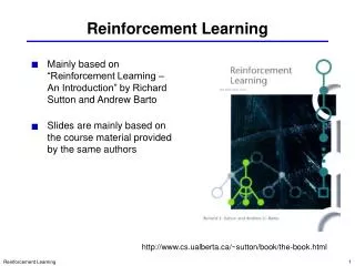
References • Sutton, R.S. and Barto, A.G. (1998).Reinforcement Learning- An Introduction. • Hastie, T., Tibshirani, R. and Friedman, J. (2001).The Elements of Statistical Learning-Data Mining, Inference and Prediction. • Murphy, S.A. (2003). Optimal Dynamic Treatment Regimes. JRSS-B. • Blatt, D., Murphy, S.A. and Zhu, J. (2004). A-Learning for Approximate Planning. • Murphy, S.A. (2004). A Generalization Error for Q-Learning.

