Reinforcement Learning
390 likes | 822 Vues
Reinforcement Learning. Problem: Find values for fixed policy (policy evaluation) Model-based learning : Learn the model, solve for values Model-free learning : Solve for values directly (by sampling). The Story So Far: MDPs and RL. Techniques:. Things we know how to do:.

Reinforcement Learning
E N D
Presentation Transcript
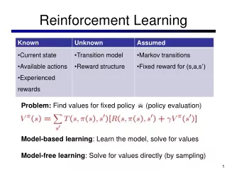
Reinforcement Learning Problem: Find values for fixed policy (policy evaluation) Model-based learning: Learn the model, solve for values Model-free learning: Solve for values directly (by sampling)
The Story So Far: MDPs and RL Techniques: Things we know how to do: • If we know the MDP • Compute V*, Q*, * exactly • Evaluate a fixed policy • If we don’t know the MDP • We can estimate the MDP then solve • We can estimate V for a fixed policy • We can estimate Q*(s,a) for the optimal policy while executing an exploration policy • Model-based DPs • Value and policy Iteration • Policy evaluation • Model-based RL • Model-free RL: • Value learning • Q-learning
Recap: Optimal Utilities • The utility of a state s: V*(s) = expected utility starting in s and acting optimally • The utility of a q-state (s,a): Q*(s,a) = expected utility starting in s, taking action a and thereafter acting optimally • The optimal policy: *(s) = optimal action from state s s is a state s a (s, a) is a q-state s, a (s,a,s’) is a transition s,a,s’ s’
Temporal-Difference Learning • Big idea: learn from every experience! • Update V(s) each time we experience (s,a,s’,r) • Likely s’ will contribute updates more often • Temporal difference learning • Policy still fixed! • Move values toward value of whatever successor occurs: running average! s (s) s, (s) s’ Sample of V(s): Update to V(s): Same update:
Example: TD Policy Evaluation (1,1) up -1 (1,2) up -1 (1,2) up -1 (1,3) right -1 (2,3) right -1 (3,3) right -1 (3,2) up -1 (3,3) right -1 (4,3) exit +100 (done) (1,1) up -1 (1,2) up -1 (1,3) right -1 (2,3) right -1 (3,3) right -1 (3,2) up -1 (4,2) exit -100 (done) Take = 1, = 0.5
s a s, a s,a,s’ s’ Problems with TD Value Learning • TD value leaning is a model-free way to do policy evaluation • However, if we want to turn values into a (new) policy, we’re sunk: • Idea: learn Q-values directly • Makes action selection model-free too!
Active Learning • Full reinforcement learning • You don’t know the transitions T(s,a,s’) • You don’t know the rewards R(s,a,s’) • You can choose any actions you like • Goal: learn the optimal policy • … what value iteration did! • In this case: • Learner makes choices! • Fundamental tradeoff: exploration vs. exploitation • This is NOT offline planning! You actually take actions in the world and find out what happens…
Model-Based Active Learning • In general, want to learn the optimal policy, not evaluate a fixed policy • Idea: adaptive dynamic programming • Learn an initial model of the environment: • Solve for the optimal policy for this model (value or policy iteration) • Refine model through experience and repeat • Crucial: we have to make sure we actually learn about all of the model
Example: Greedy ADP • Imagine we find the lower path to the good exit first • Some states will never be visited following this policy from (1,1) • We’ll keep re-using this policy because following it never collects the regions of the model we need to learn the optimal policy ? ?
What Went Wrong? • Problem with following optimal policy for current model: • Never learn about better regions of the space if current policy neglects them • Fundamental tradeoff: exploration vs. exploitation • Exploration: must take actions with suboptimal estimates to discover new rewards and increase eventual utility • Exploitation: once the true optimal policy is learned, exploration reduces utility • Systems must explore in the beginning and exploit in the limit ? ?
Detour: Q-Value Iteration • Value iteration: find successive approx optimal values • Start with V0*(s) = 0, which we know is right (why?) • Given Vi*, calculate the values for all states for depth i+1: • But Q-values are more useful! • Start with Q0*(s,a) = 0, which we know is right (why?) • Given Qi*, calculate the q-values for all q-states for depth i+1:
Q-Learning • We’d like to do Q-value updates to each Q-state: • But can’t compute this update without knowing T, R • Instead, compute average as we go • Receive a sample transition (s,a,r,s’) • This sample suggests • But we want to average over results from (s,a) (Why?) • So keep a running average
Q-Learning Properties • Will converge to optimal policy • If you explore enough (i.e. visit each q-state many times) • If you make the learning rate small enough • Basically doesn’t matter how you select actions (!) • Off-policy learning: learns optimal q-values, not the values of the policy you are following
Exploration / Exploitation • Several schemes for forcing exploration • Simplest: random actions ( greedy) • Every time step, flip a coin • With probability , act randomly • With probability 1-, act according to current policy • Regret: expected gap between rewards during learning and rewards from optimal action • Q-learning with random actions will converge to optimal values, but possibly very slowly, and will get low rewards on the way • Results will be optimal but regret will be large • How to make regret small?
Exploration Functions • When to explore • Random actions: explore a fixed amount • Better ideas: explore areas whose badness is not (yet) established, explore less over time • One way: exploration function • Takes a value estimate and a count, and returns an optimistic utility, e.g. (exact form not important)
Q-Learning • Q-learning produces tables of q-values:
Q-Learning • In realistic situations, we cannot possibly learn about every single state! • Too many states to visit them all in training • Too many states to hold the q-tables in memory • Instead, we want to generalize: • Learn about some small number of training states from experience • Generalize that experience to new, similar states • This is a fundamental idea in machine learning, and we’ll see it over and over again
Example: Pacman • Let’s say we discover through experience that this state is bad: • In naïve q learning, we know nothing about this state or its q states: • Or even this one!
Feature-Based Representations • Solution: describe a state using a vector of features (properties) • Features are functions from states to real numbers (often 0/1) that capture important properties of the state • Example features: • Distance to closest ghost • Distance to closest dot • Number of ghosts • 1 / (dist to dot)2 • Is Pacman in a tunnel? (0/1) • …… etc. • Is it the exact state on this slide? • Can also describe a q-state (s, a) with features (e.g. action moves closer to food)
Linear Feature Functions • Using a feature representation, we can write a q function (or value function) for any state using a few weights: • Advantage: our experience is summed up in a few powerful numbers • Disadvantage: states may share features but actually be very different in value!
Function Approximation • Q-learning with linear q-functions: • Intuitive interpretation: • Adjust weights of active features • E.g. if something unexpectedly bad happens, disprefer all states with that state’s features • Formal justification: online least squares Exact Q’s Approximate Q’s
26 24 22 20 30 40 20 30 20 10 10 0 0 Linear Regression 40 20 0 0 20 Prediction Prediction
Overfitting 30 25 Degree 15 polynomial 20 15 10 5 0 -5 -10 -15 0 2 4 6 8 10 12 14 16 18 20
Policy Search • Problem: often the feature-based policies that work well aren’t the ones that approximate V / Q best • E.g. your value functions from project 2 were probably horrible estimates of future rewards, but they still produced good decisions • We’ll see this distinction between modeling and prediction again later in the course • Solution: learn the policy that maximizes rewards rather than the value that predicts rewards • This is the idea behind policy search, such as what controlled the upside-down helicopter
Policy Search • Simplest policy search: • Start with an initial linear value function or q-function • Nudge each feature weight up and down and see if your policy is better than before • Problems: • How do we tell the policy got better? • Need to run many sample episodes! • If there are a lot of features, this can be impractical
