Lowest-Cost Routing
650 likes | 786 Vues
Lowest-Cost Routing. EE 122: Intro to Communication Networks Fall 2010 (MW 4-5:30 in 101 Barker) Scott Shenker TAs: Sameer Agarwal, Sara Alspaugh, Igor Ganichev, Prayag Narula http://inst.eecs.berkeley.edu/~ee122/

Lowest-Cost Routing
E N D
Presentation Transcript
Lowest-Cost Routing EE 122: Intro to Communication Networks Fall 2010 (MW 4-5:30 in 101 Barker) Scott Shenker TAs: Sameer Agarwal, Sara Alspaugh, Igor Ganichev, Prayag Narula http://inst.eecs.berkeley.edu/~ee122/ Materials with thanks to Jennifer Rexford, Ion Stoica, Vern Paxsonand other colleagues at Princeton and UC Berkeley
Announcements • Revision to lecture schedule • Advanced topics on routing • Revision to homework schedule • 3a: get midterm questions right • 3b: new topics • Changes to class structure • 5 minute “technology break” • Administrivia right after break • Group problem solving (when possible) • Sit next to smart people
Goals of Today’s Lecture • Routing overview: • Routing vs. forwarding • Routing topics • Link-state routing (Dijkstra’s algorithm) • Distance-vector routing (Bellman-Ford)
Forwarding vs. Routing • Forwarding: “data plane” • Directing a data packet to an outgoing link • Individual router using a forwarding table • Routing: “control plane” • Computing paths the packets will follow • Routers talking amongst themselves • Jointly creating a forwarding table
Why Does Routing Matter? • Routing provides connectivity! • Without routing, the network doesn’t function • Routing finds “good” paths • Propagation delay, throughput, packet loss • Routing allows network to tolerate failures • Limits packet loss during disruptions • Routing can also provide “Traffic Engineering” • Balance traffic over the routers and links • Avoid congestion by directing traffic to lightly-loaded links • (Not covered today)
Three Lectures on Routing • Today: Lowest-cost routing • Simple algorithms, basic issues • Wednesday: Policy-based routing • Interdomain routing • Monday: Advanced topics • Traffic engineering • Improved resilience • What future routing algorithms might look like….
Link State Routing E.g. Algorithm: Dijkstra E.g. Protocol: OSPF Distance Vector Routing E.g. Algorithm: Bellman-Ford E.g. Protocol: RIP Routing Requires Knowing Network • Centralized global state • Single entity knows the complete network structure • Can calculate all routes centrally • Problems with this approach? • Distributed global state • Every router knows the complete network structure • Independently calculates routes • Problems with this approach? • Distributed global computation • Every router knows only about its neighboring routers • Participates in global joint calculation of routes • Problems with this approach?
5 3 5 2 2 1 3 1 2 1 C D A B E F Modeling a Network • Modeled as a graph • Routers nodes • Link edges • Possible edge costs • Hop • Delay • Congestion level • …. • Goal of Routing • Determine “good” path from source to destination • “Good” usually means the lowest “cost” path • Where cost is usually hop-count or latency
From Model to Reality • In reality, attach prefixes to nodes • Calculate routing tables in terms of prefixes • But ignore this for now….. • Just calculate paths between routers
Why Isn’t All Routing Lowest-Cost? • Lowest-cost routing assumes all nodes evaluate paths the same way • i.e., use same “cost” metric • Interdomain routing: • Different domains care about different things • Can exercise general “policy” goals • Requires very different route computation • Talk about on Wednesday….
Link State Routing • Each router has complete network picture • Topology • Link costs • How does each router get the global state? • Each router reliably floods information about its neighbors to every other router (more later) • Each router independently calculates the shortest path from itself to every other router • Using, for example, Dijkstra’s Algorithm
Host C Host D Host A N2 N1 N3 N5 Host B Host E N4 N6 N7 Link State: Control Traffic • Each node floods its local information • Each node ends up knowing the entire network topology node
C C C C C C C A A A A A A A D D D D D D D Host C Host D Host A B B B B B B B E E E E E E E N2 N1 N3 N5 Host B Host E N4 N6 N7 Link State: Node State
Dijkstra’s Shortest Path Algorithm • INPUT: • Network topology (graph), with link costs • OUTPUT: • Least cost paths from one node to all other nodes • Produces “tree” of routes (why?)
c(i,j): link cost from node i to j; cost infinite if not direct neighbors; ≥ 0 D(v): current value of cost of path from source to destination v p(v): predecessor node along path from source to v, that is next to v S: set of nodes whose least cost path definitively known D C A E B F 5 3 5 2 2 1 3 1 2 1 Notation Source
Dijsktra’s Algorithm • c(i,j): link cost from node i to j • D(v): current cost source v • p(v): predecessor node along path from source to v, that is next to v • S: set of nodes whose least cost path definitively known 1 Initialization: 2 S = {A}; 3 for all nodes v 4 if v adjacent to A 5 then D(v) = c(A,v); 6 else D(v) = ; 7 8 Loop 9 find w not in S such that D(w) is a minimum; 10 add w to S; 11 update D(v) for all v adjacent to w and not in S: 12 if D(w) + c(w,v) < D(v) then // w gives us a shorter path to v than we’ve found so far 13 D(v) = D(w) + c(w,v); p(v) = w; 14 until all nodes in S;
D C A E B F 5 3 5 2 2 1 3 1 2 1 Example: Dijkstra’s Algorithm D(B),p(B) 2,A D(D),p(D) 1,A D(C),p(C) 5,A D(E),p(E) Step 0 1 2 3 4 5 start S A D(F),p(F) 1 Initialization: 2 S = {A}; 3 for all nodes v 4 if v adjacent to A 5 then D(v) = c(A,v); 6 else D(v) = ; …
… • 8 Loop • 9 find w not in S s.t. D(w) is a minimum; • 10 add w to S; • update D(v) for all v adjacent • to w and not in S: • If D(w) + c(w,v) < D(v) then • D(v) = D(w) + c(w,v); p(v) = w; • 14 until all nodes in S; D C A E B F 5 3 5 2 2 1 3 1 2 1 Example: Dijkstra’s Algorithm D(B),p(B) 2,A D(D),p(D) 1,A D(C),p(C) 5,A D(E),p(E) Step 0 1 2 3 4 5 start S A D(F),p(F)
… • 8 Loop • 9 find w not in S s.t. D(w) is a minimum; • 10 add w to S; • update D(v) for all v adjacent • to w and not in S: • If D(w) + c(w,v) < D(v) then • D(v) = D(w) + c(w,v); p(v) = w; • 14 until all nodes in S; C D E A B F Example: Dijkstra’s Algorithm D(B),p(B) 2,A D(D),p(D) 1,A D(C),p(C) 5,A D(E),p(E) Step 0 1 2 3 4 5 start S A AD D(F),p(F) 5 3 5 2 2 1 3 1 2 1
… • 8 Loop • 9 find w not in S s.t. D(w) is a minimum; • 10 add w to S; • update D(v) for all v adjacent • to w and not in S: • If D(w) + c(w,v) < D(v) then • D(v) = D(w) + c(w,v); p(v) = w; • 14 until all nodes in S; C D E A B F Example: Dijkstra’s Algorithm D(B),p(B) 2,A D(D),p(D) 1,A D(C),p(C) 5,A 4,D D(E),p(E) 2,D Step 0 1 2 3 4 5 start S A AD D(F),p(F) 5 3 5 2 2 1 3 1 2 1
… • 8 Loop • 9 find w not in S s.t. D(w) is a minimum; • 10 add w to S; • update D(v) for all v adjacent • to w and not in S: • If D(w) + c(w,v) < D(v) then • D(v) = D(w) + c(w,v); p(v) = w; • 14 until all nodes in S; C D E A B F Example: Dijkstra’s Algorithm D(B),p(B) 2,A D(D),p(D) 1,A D(C),p(C) 5,A 4,D 3,E D(E),p(E) 2,D Step 0 1 2 3 4 5 start S A AD ADE D(F),p(F) 4,E 5 3 5 2 2 1 3 1 2 1
… • 8 Loop • 9 find w not in S s.t. D(w) is a minimum; • 10 add w to S; • update D(v) for all v adjacent • to w and not in S: • If D(w) + c(w,v) < D(v) then • D(v) = D(w) + c(w,v); p(v) = w; • 14 until all nodes in S; C D E A B F Example: Dijkstra’s Algorithm D(B),p(B) 2,A D(D),p(D) 1,A D(C),p(C) 5,A 4,D 3,E D(E),p(E) 2,D Step 0 1 2 3 4 5 start S A AD ADE ADEB D(F),p(F) 4,E 5 3 5 2 2 1 3 1 2 1
… • 8 Loop • 9 find w not in S s.t. D(w) is a minimum; • 10 add w to S; • update D(v) for all v adjacent • to w and not in S: • If D(w) + c(w,v) < D(v) then • D(v) = D(w) + c(w,v); p(v) = w; • 14 until all nodes in S; C D E A B F Example: Dijkstra’s Algorithm D(B),p(B) 2,A D(D),p(D) 1,A D(C),p(C) 5,A 4,D 3,E D(E),p(E) 2,D Step 0 1 2 3 4 5 start S A AD ADE ADEB ADEBC D(F),p(F) 4,E 5 3 5 2 2 1 3 1 2 1
… • 8 Loop • 9 find w not in S s.t. D(w) is a minimum; • 10 add w to S; • update D(v) for all v adjacent • to w and not in S: • If D(w) + c(w,v) < D(v) then • D(v) = D(w) + c(w,v); p(v) = w; • 14 until all nodes in S; C D E A B F 5 3 5 2 2 1 3 1 2 1 Example: Dijkstra’s Algorithm D(B),p(B) 2,A D(D),p(D) 1,A D(C),p(C) 5,A 4,D 3,E D(E),p(E) 2,D Step 0 1 2 3 4 5 start S A AD ADE ADEB ADEBC ADEBCF D(F),p(F) 4,E
D C A E B F 5 3 5 2 2 1 3 1 2 1 Example: Dijkstra’s Algorithm D(B),p(B) 2,A D(D),p(D) 1,A D(C),p(C) 5,A 4,D 3,E D(E),p(E) 2,D Step 0 1 2 3 4 5 start S A AD ADE ADEB ADEBC ADEBCF D(F),p(F) 4,E To determine path A C (say), work backward from C via p(v)
D C A E B F 5 3 5 2 2 1 3 1 2 1 The Forwarding Table • Running Dijkstra at node A gives the shortest path from A to all destinations • We then construct the forwarding table
Complexity • How much processing does running the Dijkstra algorithm take? • Assume a network consisting of N nodes • Each iteration: check all nodes w not in S • N(N+1)/2 comparisons: O(N2) • More efficient implementations: O(N log(N))
X A X A C B D C B D (a) (b) X A X A C B D C B D (c) (d) Obtaining Global State • Flooding • Each router sends link-state information out its links • The next node sends it out through all of its links • except the one where the information arrived • Note: need to remember previous msgs & suppress duplicates!
Flooding the Link State • Reliable flooding • Ensure all nodes receive link-state information • Ensure all nodes use the latest version • Challenges • Packet loss • Out-of-order arrival • Solutions • Acknowledgments and retransmissions • Sequence numbers
When to Initiate Flooding • Topology change • Link or node failure • Link or node recovery • Configuration change • Link cost change • Potential problems with making cost dynamic! • Periodically • Refresh the link-state information • Typically (say) 30 minutes • Corrects for possible corruption of the data
e C C C C C D D D D D B A B A B A B B A A 0 2+e 2+e 2+e 0 0 0 0 1 1 1+e 1+e 1 1+e 0 e 0 0 … recompute … recompute routing … recompute Oscillating Load-Dependent Routing • Assume link cost = amount of carried traffic • All traffic sent to A 1 1+e 0 0 e 0 1 1 initially 0 0 0 0 Very Hard to Avoid Oscillations!
Detecting Topology Changes • Beaconing • Periodic “hello” messages in both directions • Detect a failure after a few missed “hellos” • Performance trade-offs • Detection speed • Overhead on link bandwidth and CPU • Likelihood of false detection “hello”
Convergence • Getting consistent routing information to all nodes • E.g., all nodes having the same link-state database • Consistent forwarding after convergence • All nodes have the same link-state database • All nodes forward packets on shortest paths • The next router on the path forwards to the next hop
Convergence Delay • Time elapsed before every router has a consistent picture of the network • Sources of convergence delay • Detection latency • Flooding of link-state information • Recomputation of forwarding tables • Performance during convergence period • Lost packets due to blackholes and TTL expiry • Looping packets consuming resources • Out-of-order packets reaching the destination • Very bad for VoIP, online gaming, and video
Reducing Convergence Delay • Faster detection • Smaller hello timers • Link-layer technologies that can detect failures • Faster flooding • Flooding immediately • Sending link-state packets with high-priority • Faster computation • Faster processors on the routers • Incremental Dijkstra algorithm • Faster forwarding-table update • Data structures supporting incremental updates
D C D C A A E E B B F F Loop! Transient Disruptions • Inconsistent link-state database • Some routers know about failure before others • The shortest paths are no longer consistent • Can cause transient forwarding loops E thinks that thisis the path to C A and D think that thisis the path to C
Area 2 Area 3 Scaling Link-State Routing • Overhead of link-state routing • Flooding link-state packets throughout the network • Running Dijkstra’s shortest-path algorithm • Becomes unscalable when 100s of routers • Introducing hierarchy through “areas” Area 1 Area 0 area border router Area 4
Link-State Routing Is Conceptually Simple • Each router keeps track of its incident links • Link cost, and whether the link is up or down • Each router broadcasts the link state • To give every router a complete view of the graph • Each router runs Dijkstra’s algorithm • Compute shortest paths, then construct forwarding table • Example protocols • Open Shortest Path First (OSPF) • Intermediate System – Intermediate System (IS-IS) • Challenges: scaling, transient disruptions • Any ideas for improvement?
Question • Why use different routing algorithms at L2 and L3? • Is Link-State “plug-and-play”? • Could we make it “plug-and-play?”
5 Minute Break Questions Before We Proceed?
Feedback on Course • Course moving: • Too slowly: 13% • Too quickly: 30% • OK: 57% • Lectures should be: • Harder: 18% • Easier: 26% • Same: 56% • Homework should be: • Harder: 33% • Easier: 13% • Same: 54% • Include History/Politics: • Yes: 76% • Include worked ex’s: • Yes: 82% • Project is: • Too easy: 11% • Too hard: 33% • OK: 56% • Support in Section • Yes: 80% • Don’t go: 12%
Selected Comments • Use newsgroups • Weekly homeworks • Relate project to course • Don't skip break • Test too easy • Bspace is evil • “Cancel the project and final, buy us dinner” • “Make lectures less boring”
More Scalable Routing Algorithms? • Avoid need for global state consistency • Just focus on computing routes • Distribute the computation, not the state….
Distance Vector Routing • Each router knows the links to its neighbors • Does not flood this information to the whole network • Each router has provisional “shortest path” • E.g.: Router A: “I can get to router B with cost 11 via next hop router D” • Routers exchange this information with their neighboring routers • Again, no flooding the whole network • Routers update their idea of the best path using info from neighbors • This iterative process converges with set of shortest paths
Host C Host D Host A N2 N1 N3 N5 Host B Host E N4 N6 N7 Information Flow in Distance Vector
Host C Host D Host A N2 N1 N3 N5 Host B Host E N4 N6 N7 Information Flow in Distance Vector
Host C Host D Host A N2 N1 N3 N5 Host B Host E N4 N6 N7 Information Flow in Distance Vector
Bellman-Ford Algorithm • INPUT: • Link costs to each neighbor • Not full topology • OUTPUT: • Next hop to each destination and the corresponding cost • Does not give the complete path to the destination
wait for (change in local link cost or msg from neighbor) recompute distance table if least cost path to any dest has changed, notify neighbors Each node: Bellman-Ford - Overview • Each router maintains a table • Row for each possible destination • Column for each directly-attached neighbor to node • Entry in row Y and column Z of node X best known distance from X to Y, via Z as next hop = DZ(X,Y) • Each local iteration caused by: • Local link cost change • Message from neighbor • Notify neighbors only if least cost path to any destination changes • Neighbors then notify their neighbors if necessary