4.5 Dijkstra’s Algorithm

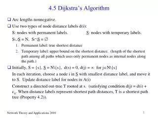
1. 4.5 Dijkstra’s Algorithm • Arc lengths nonnegative. • Use two types of node distance labels d(i): S: nodes with permanent labels. S: nodes with temporary labels. SS = N, SS =  • Permanent label: true shortest distance • Temporary label: upper bound on the shortest distance. (length of the shortest path among all paths which uses only permanent nodes as internal nodes along the path.) • Initially, S = {s}, S = N\{s}, d(s) = 0, d(j) =  for jN\{s} In each iteration, choose a node i in S with smallest distance label, and move it to S. Update distance label for nodes in A(i) Construct a directed out-tree T rooted at s. (satisfying condition d(j) = d(i) + cij. When distance labels represent shortest path distances, T is a shortest path tree (Property 4.2)).

2. Algorithm Dijkstra: begin S := ; S :=N; d(i) :=  for each node iN; d(s) := 0 and pred(s) := 0; While |S| < n do begin let iS be a node for which d(i) = min{d(j): jS}; S = S  {i}; S = S\{i}; for each (i, j)A(i) do if d(j) > d(i) + cij then d(j):= d(i) + cij and pred(j):= i; end; end

3. Ex) permanent labeling sequence: 3, 4, 2, 5, 6 2 3 5 3 4 1 2 1 6 1 1 6 7 2 4 2

4. Correctness of Dijkstra’s Algorithm: Use induction on |S|. Induction hypothesis are (1) the distance label of each node in S is optimal (2) the distance label of each node in S is the shortest path length from the source provided that each internal node in the path lies in S. Algorithm selects a node iS with smallest node label and move it to S. Need to show that d(i) is optimal. By induction hypothesis, d(i) is shortest among all paths that do not contain any node in S as an internal node. Show that the length of any path to i that may include some nodes in S as an internal node is at least d(i). Consider any path P that contains a node in S as internal node. Let k be the first such node. i Pred(i) S S P2 s k P1

5. (continued) The path P = P1 + P2. We know that d(i)  d(k) since algorithm selects node i instead of k. So length of P = d(k) + length of P2  d(i) since arc lengths are nonnegative. Hence d(i) is optimal. For the second hypothesis, observe that any such path remains the same or use node i as its last node (check this), in which case we have d(j) = d(i) + cij jS.  • Running time of Dijkstra’s algorithm • Node selection: performs n times and each iteration scans each temporarily labeled node  n + (n-1) + (n-2) + … + 1 = O(n2) • Distance updates: performs |A(i)| times for node i. Overall, iN |A(i)| = m. O(m) total time • Thm 4.4. Dijkstra’s algorithm solves the shortest path problem (with nonnegative arc lengths) in O(n2) time.

6. Reverse Dijkstra’s Algorithm: Determine a shortest path from every node in N\{t} to a sink node t. Maintain a distance d’(j) for each node j, which is an upper bound on the shortest path length from node j to node t. Use permanently labeled node set S’ and temporarily labeled node set S’. Select node j in S’ with minimum label and move it to S’. Update node labels for each incoming arc (i, j) as min { d’(i), cij + d’(j)} • Bidirectional Dijkstra’s Algorithm

7. 4.6 Dial’s Implementation • How to find a node with minimum distance label efficiently? • Property 4.5. The distance labels that Dijkstra’s algorithm designates as permanent are nondecreasing. • Primitive form of using buckets: Use nC + 1 sets, called buckets, numbered 0, 1, … , nC. (C:largest arc length) bucket k stores temporary nodes with label value k (use doubly linked list in each bucket). Let content(k) represent the contents of bucket k. Scan from 0  nC. The first nonempty bucket (say k) contains nodes with minimum distance label. Remove a node from bucket kand update the node label d1  d2 (remove the node from bucket d1 and add to bucket d2 ) • Running time: O(m+nC) (pseudopolynomial) O(m) for distance update, O(nC) for finding minimum label

8. Dial’s implementation needs large memory. remedy: maintain C+1 buckets with modulus operation. • Property 4.6. At the beginning of an iteration, if d(i) is the new permanent label, then for all temporary labels d(j), jS, we have d(j)  d(i) + C at the end of the iteration. Pf) (1) d(l)  d(i) for lS (property 4.5). (2) For any finitely labeled node jS, d(j) = d(l) + clj for some lS. Therefore, d(j) = d(l) + clj  d(i) + C  • All temporary labels lie between d(i) and d(i)+C.  Use C+1 buckets in modular fashion. • Use buckets numbered 0, 1, 2, … , C. Store temporary node j with label d(j) in bucket d(j) mod(C+1). Bucket(k) stores nodes with labels k, k + (C+1), k + 2(C+1), and so on. If bucket k stores a node with minimum distance label, then buckets k+1, k+2, … , C, 0, 1, 2, … , k-1 store nodes in increasing value of the distance labels.

9. Examine the buckets sequentially, in a wraparound fashion, to identify the first nonempty bucket. In the next iteration, it reexamines the buckets starting at the place where it left off previously • Running time still O(m+nC). Works well in practice (when C is modest).

10. 4.7 Heap Implementations • Heap (priority queue): data structure which allows some operations on the set can be performed efficiently. (binary heap, d-heap, …) Key value 5 5 7 6 7 4 swap 11 12 4 8 11 12 6 8 9 9 • Each node has node label and a key value (weight). • Place nodes from top  bottom, left  right (in array).

11. Property A.1 • At most dk nodes have depth k. • At most (dk+1-1)/(d-1) nodes have depth between 0 and k. • The depth of a d-heap containing n nodes is at most logdn. • Property A.2 • The predecessor of the node in array(i) is contained in position (i-1)/2. • The successors of the node in array(i) is in positions id-d+2, … , id+1. • Property A.3 (invariant 1) key(i)  key(j) for jSUCC(i) (always maintain this property at the end of an operation.)

12. Basic operations: • swap(i, j): interchange node i and j O(1) time • siftup(i): while key(i) < key(pred(i)) do swap(i, pred(i)) O(logdn) time • siftdown(i): while key(i) > key(minchild(i)) do swap(i, minchild(i)) O(dlogdn) time • Heap operations: • create-heap(H): Create an empty heap • find-min(i, H): Find and return an object i of minimum key O(1) • insert(i, H): Insert a new object i with a predefined key. Insert at the end, then siftup(i) O(logdn) • decrease-key(value, i, H): Reduce the key of object i from its current value to value which is smaller. Use siftup(i) O(logdn) • increase-key(value, i, H): Use siftdown(i) O(dlogdn) • delete-min(i, H): Delete an object i of minimum key. Use swap(root, last), then last = last – 1, siftdown(root) O(dlogdn) • delete(i, H): Delete object i. Use swap(i, last), then last = last – 1, siftdown(i) O(dlogdn)

13. Heap implementation of Dijkstra’s algorithm: begin create-heap(H) d(j) :=  for all jN; d(s) := 0 and pred(s) := 0; insert(s, H); While H   do begin find-min(i, H); delete-min(i, H); for each (i, j)A(i) do begin value := d(i) + cij; if d(j) > value then if d(j) =  then d(j) := value, pred(j) := i, and insert(j, H) else set d(j):=value, pred(j):=i, decrease-key(value, i, H); if d(j) > d(i) + cij then d(j):= d(i) + cij and pred(j):= i; end end; end

14. Heap implementation: find-min, delete-min, insert: O(n) steps decrease-key: O(m) steps • Binary heap implementation: delete-min, insert, decrease-key: O(log n) find-min: O(1) Total time is O(m log n) • d-heap implementation: insert, decrease-key: O(logd n) delete-min: O(d logd n), find-min: O(1) Total time is O(m logd n + nd logd n) • Optimal d = max{2, m/n} → O(m logd n)

15. Fibonacci heap implementation: set of rooted trees. performs every heap operation in O(1) amortized time, except delete-min, which requires O(log n) time . → O(m + n log n) • Johnson’s implementation: O(log log C) time to perform each heap operation. → O(m log log C)

16. 4.8 Radix Heap Implementation • Using buckets • Original Dijkstra: 1 bucket • Dial’s implementation: (1+nC) buckets • Radix heap: inbetween using heap idea • A bucket can store nodes with label values in some range. • - The widths of the buckets are 1, 1, 2, 4, 8, 16, … , so that the number of buckets is O(log(nC)). - Note that the width of bucket k is the same as the sum of widths of buckets 0, 1, 2, … , k-1. Hence the nodes in bucket k can be redistributed to buckets 0, 1, 2, … , k-1. - Dynamically modify the ranges of the buckets and reallocate nodes. The node with the smallest temporary label is stored in the first bucket.

17. Initial bucket ranges: • range(0) = [0] range(1) = [1] range(2) = [2, 3] range(3) = [4, 7] range(4) = [8, 15] … range(K) = [2K-1, 2K – 1], where K = log(nC) Bucket i contains nodes (content(i)) with labels within the range(i)

18. Steps of algorithm: Find minimum label from the first nonempty bucket, say i. Suppose range(i) = [l, u] and the minimum label is dmin. Then labels in range(i) lies in [dmin, u]. Redistribute this range to buckets 0, 1, 2, … , i. Then we have new ranges, range(0) = [dmin], range(1) = [dmin+1], range(2) = [dmin+2, dmin+3], … , and range(i) =  now. Then bucket 0 always has the smallest label. • Update the node labels and place them in appropriate buckets. Note that the node label never increases, hence scan the buckets from right to left starting from the current bucket until we identify correct range. (Number of bucket changes for each node is at most K)

19. Running time O(m+nK) for node movement: m for the number of distance updates, and nK for node movement. O(nK) for node selection: O(K) time to identify the first nonempty bucket, n iterations. O(nK) for redistribution of ranges. Hence overall running time is O(m+nK) or O(m + n log(nC)) • May use 1+log C buckets as in Dial’s. Then O(m + n log C) • Using Fibonacci heap within radix heap → O(m + n(log C)1/2) • Best running time: O(min{m + n log n, m log log C, m + n(log C)1/2})