CSE332: Data Abstractions Lecture 26: Minimum Spanning Trees
580 likes | 770 Vues
CSE332: Data Abstractions Lecture 26: Minimum Spanning Trees. Dan Grossman Spring 2010. “Scheduling note”. “We now return to our interrupted program” on graphs Last “graph lecture” was lecture 17 Shortest-path problem Dijkstra’s algorithm for graphs with non-negative weights

CSE332: Data Abstractions Lecture 26: Minimum Spanning Trees
E N D
Presentation Transcript
CSE332: Data AbstractionsLecture 26: Minimum Spanning Trees Dan Grossman Spring 2010
“Scheduling note” • “We now return to our interrupted program” on graphs • Last “graph lecture” was lecture 17 • Shortest-path problem • Dijkstra’s algorithm for graphs with non-negative weights • Why this strange schedule? • Needed to do parallelism and concurrency in time for project 3 and homeworks 6 and 7 • But cannot delay all of graphs because of the CSE312 co-requisite • So: not the most logical order, but hopefully not a big deal CSE332: Data Abstractions
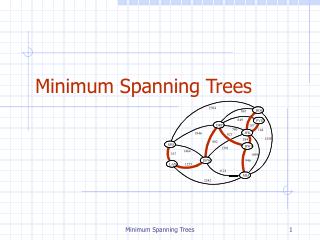
Spanning trees • A simple problem: Given a connected graph G=(V,E), find a minimal subset of the edges such that the graph is still connected • A graph G2=(V,E2) such that G2 is connected and removing any edge from E2 makes G2 disconnected CSE332: Data Abstractions
Observations • Any solution to this problem is a tree • Recall a tree does not need a root; just means acyclic • For any cycle, could remove an edge and still be connected • Solution not unique unless original graph was already a tree • Problem ill-defined if original graph not connected • A tree with |V| nodes has |V|-1 edges • So every solution to the spanning tree problem has |V|-1 edges CSE332: Data Abstractions
Motivation A spanning tree connects all the nodes with as few edges as possible • Example: A “phone tree” so everybody gets the message and no unnecessary calls get made • Bad example since would prefer a balanced tree In most compelling uses, we have a weighted undirected graph and we want a tree of least total cost • Example: Electrical wiring for a house or clock wires on a chip • Example: A road network if you cared about asphalt cost rather than travel time This is the minimum spanning tree problem • Will do that next, after intuition from the simpler case CSE332: Data Abstractions
Two approaches Different algorithmic approaches to the spanning-tree problem: • Do a graph traversal (e.g., depth-first search, but any traversal will do), keeping track of edges that form a tree • Iterate through edges; add to output any edge that doesn’t create a cycle CSE332: Data Abstractions
Spanning tree via DFS spanning_tree(Graph G) { for each node i: i.marked = false for some node i: f(i) } f(Node i) { i.marked = true for each j adjacent to i: if(!j.marked) { add(i,j) to output f(j) // DFS } } Correctness: DFS reaches each node. We add one edge to connect it to the already visited nodes. Order affects result, not correctness. Time: O(|E|) CSE332: Data Abstractions
Example Stack f(1) 2 1 3 7 4 6 5 Output: CSE332: Data Abstractions
Example Stack f(1) f(2) 2 1 3 7 4 6 5 Output: (1,2) CSE332: Data Abstractions
Example Stack f(1) f(2) f(7) 2 1 3 7 4 6 5 Output: (1,2), (2,7) CSE332: Data Abstractions
Example Stack f(1) f(2) f(7) f(5) 2 1 3 7 4 6 5 Output: (1,2), (2,7), (7,5) CSE332: Data Abstractions
Example Stack f(1) f(2) f(7) f(5) f(4) 2 1 3 7 4 6 5 Output: (1,2), (2,7), (7,5), (5,4) CSE332: Data Abstractions
Example Stack f(1) f(2) f(7) f(5) f(4) f(3) 2 1 3 7 4 6 5 Output: (1,2), (2,7), (7,5), (5,4),(4,3) CSE332: Data Abstractions
Example Stack f(1) f(2) f(7) f(5) f(4) f(6) f(3) 2 1 3 7 4 6 5 Output: (1,2), (2,7), (7,5), (5,4), (4,3), (5,6) CSE332: Data Abstractions
Example Stack f(1) f(2) f(7) f(5) f(4) f(6) f(3) 2 1 3 7 4 6 5 Output: (1,2), (2,7), (7,5), (5,4), (4,3), (5,6) CSE332: Data Abstractions
Second approach Iterate through edges; output any edge that doesn’t create a cycle Correctness (hand-wavy): • Goal is to build an acyclic connected graph • When we don’t add an edge, adding it would not connect any nodes that aren’t already connected in the output • So we won’t end up with less than a spanning tree Efficiency: • Depends on how quickly you can detect cycles • Reconsider after the example CSE332: Data Abstractions
Example Edges in some arbitrary order: (1,2), (3,4), (5,6), (5,7),(1,5), (1,6), (2,7), (2,3), (4,5), (4,7) 2 1 3 7 4 6 5 Output: CSE332: Data Abstractions
Example Edges in some arbitrary order: (1,2), (3,4), (5,6), (5,7),(1,5), (1,6), (2,7), (2,3), (4,5), (4,7) 2 1 3 7 4 6 5 Output: (1,2) CSE332: Data Abstractions
Example Edges in some arbitrary order: (1,2), (3,4), (5,6), (5,7),(1,5), (1,6), (2,7), (2,3), (4,5), (4,7) 2 1 3 7 4 6 5 Output: (1,2), (3,4) CSE332: Data Abstractions
Example Edges in some arbitrary order: (1,2), (3,4), (5,6), (5,7),(1,5), (1,6), (2,7), (2,3), (4,5), (4,7) 2 1 3 7 4 6 5 Output: (1,2), (3,4), (5,6), CSE332: Data Abstractions
Example Edges in some arbitrary order: (1,2), (3,4), (5,6), (5,7),(1,5), (1,6), (2,7), (2,3), (4,5), (4,7) 2 1 3 7 4 6 5 Output: (1,2), (3,4), (5,6), (5,7) CSE332: Data Abstractions
Example Edges in some arbitrary order: (1,2), (3,4), (5,6), (5,7), (1,5), (1,6), (2,7), (2,3), (4,5), (4,7) 2 1 3 7 4 6 5 Output: (1,2), (3,4), (5,6), (5,7), (1,5) CSE332: Data Abstractions
Example Edges in some arbitrary order: (1,2), (3,4), (5,6), (5,7), (1,5), (1,6), (2,7), (2,3), (4,5), (4,7) 2 1 3 7 4 6 5 Output: (1,2), (3,4), (5,6), (5,7), (1,5) CSE332: Data Abstractions
Example Edges in some arbitrary order: (1,2), (3,4), (5,6), (5,7), (1,5), (1,6), (2,7), (2,3), (4,5), (4,7) 2 1 3 7 4 6 5 Output: (1,2), (3,4), (5,6), (5,7), (1,5) CSE332: Data Abstractions
Example Edges in some arbitrary order: (1,2), (3,4), (5,6), (5,7), (1,5), (1,6), (2,7), (2,3), (4,5), (4,7) 2 1 3 7 4 6 Can stop once we have |V|-1 edges 5 Output: (1,2), (3,4), (5,6), (5,7), (1,5), (2,3) CSE332: Data Abstractions
Cycle detection • To decide if an edge could form a cycle is O(|V|) since we may need to traverse all edges already in the output • So overall algorithm would be O(|V||E|) • But there is a faster way using the disjoint-set ADT • Initially, each item is in its own 1-element set • find(u,v): are u and v in the same set? • union(u,v): union (combine) the sets u and v are in (Operations often presented slightly differently) CSE332: Data Abstractions
Using disjoint-set Can use a disjoint-set implementation in our spanning-tree algorithm to detect cycles: Invariant: u and v are connected in output-so-far iff uand v in the same set • Initially, each node is in its own set • When processing edge (u,v): • If find(u,v), then do not add the edge • Else add the edge and union(u,v) CSE332: Data Abstractions
Why do this? • Using an ADT someone else wrote is easier than writing your own cycle detection • It is also more efficient • Chapter 8 of your textbook gives several implementations of different sophistication and asymptotic complexity • A slightly clever and easy-to-implement one is O(logn) for find and union (as we defined the operations here) • Lets our spanning tree algorithm be O(|E|log|V|) [We skipped disjoint-sets as an example of “sometimes knowing-an-ADT-exists and you-can-learn-it-on-your-own suffices”] CSE332: Data Abstractions
Summary so far The spanning-tree problem • Add nodes to partial tree approach is O(|E|) • Add acyclic edges approach is O(|E|log|V|) • Using the disjoint-set ADT “as a black box” But really want to solve the minimum-spanning-tree problem • Given a weighted undirected graph, give a spanning tree of minimum weight • Same two approaches will work with minor modifications • Both will be O(|E|log|V|) CSE332: Data Abstractions
Punch line Algorithm #1 Shortest-path is to Dijkstra’s Algorithm as Minimum Spanning Tree is to Prim’s Algorithm (Both based on expanding cloud of known vertices, basically using a priority queue instead of a DFS stack) Algorithm #2 Kruskal’s Algorithm for Minimum Spanning Tree is Exactly our 2nd approach to spanning tree but process edges in cost order CSE332: Data Abstractions
Prim’s Algorithm Idea Idea: Grow a tree by adding an edge from the “known” vertices to the “unknown” vertices. Pick the edge with the smallest weight that connects “known” to “unknown.” Recall Dijkstra “picked the edge with closest known distance to the source.” • But that’s not what we want here • Otherwise identical • Compare to slides in lecture 17 if you don’t believe me CSE332: Data Abstractions
The algorithm • For each node v, set v.cost = andv.known = false • Choose any node v. • Mark v as known • For each edge (v,u) with weight w, set u.cost=w and u.prev=v • While there are unknown nodes in the graph • Select the unknown node v with lowest cost • Mark v as known and add (v, v.prev) to output • For each edge (v,u) with weight w, if(w < u.cost) { u.cost = w; u.prev = v; } CSE332: Data Abstractions
Example 2 B A 1 1 5 2 E 1 D 1 3 5 C 6 G 2 10 F CSE332: Data Abstractions
Example 2 0 2 B A 1 1 5 2 E 1 1 D 1 3 5 C 2 6 G 2 10 F CSE332: Data Abstractions
Example 2 0 2 B A 1 1 1 5 2 E 1 1 D 1 3 5 C 2 5 6 G 2 6 10 F CSE332: Data Abstractions
Example 2 0 2 B A 1 1 1 5 2 E 1 1 D 1 3 5 C 2 5 6 G 2 2 10 F CSE332: Data Abstractions
Example 1 0 2 B A 1 1 1 5 2 E 1 1 D 1 3 5 C 2 3 6 G 2 2 10 F CSE332: Data Abstractions
Example 1 0 2 B A 1 1 1 5 2 E 1 1 D 1 3 5 C 2 3 6 G 2 2 10 F CSE332: Data Abstractions
Example 1 0 2 B A 1 1 1 5 2 E 1 1 D 1 3 5 C 2 3 6 G 2 2 10 F CSE332: Data Abstractions
Example 1 0 2 B A 1 1 1 5 2 E 1 1 D 1 3 5 C 2 3 6 G 2 2 10 F CSE332: Data Abstractions
Analysis • Correctness ?? • A bit tricky • Intuitively similar to Dijkstra • Might return to this time permitting (unlikely) • Run-time • Same as Dijkstra • O(|E|log |V|) using a priority queue CSE332: Data Abstractions
Kruskal’s Algorithm Idea: Grow a forest out of edges that do not grow a cycle, just like for the spanning tree problem. • But now consider the edges in order by weight So: • Sort edges: O(|E|log |E|) • Iterate through edges using union-find for cycle detection O(|E|log |V|) Somewhat better: • Floyd’s algorithm to build min-heap with edges O(|E|) • Iterate through edges using union-find for cycle detection and deleteMin to get next edge O(|E|log |V|) • (Not better worst-case asymptotically, but often stop long before considering all edges) CSE332: Data Abstractions
Pseudocode • Sort edges by weight (better: put in min-heap) • Each node in its own set • While output size <|V|-1 • Consider next smallest edge (u,v) • if find(u,v) indicates u and v are in different sets • output (u,v) • union(u,v) Recall invariant: u and v in same set if and only if connected in output-so-far CSE332: Data Abstractions
Example 2 B A Edges in sorted order: 1: (A,D), (C,D), (B,E), (D,E) 2: (A,B), (C,F), (A,C) 3: (E,G) 5: (D,G), (B,D) 6: (D,F) 10: (F,G) 1 1 5 2 E 1 D 1 3 5 C 6 G 2 10 F Output: Note: At each step, the union/find sets are the trees in the forest CSE332: Data Abstractions
Example 2 B A Edges in sorted order: 1: (A,D), (C,D), (B,E), (D,E) 2: (A,B), (C,F), (A,C) 3: (E,G) 5: (D,G), (B,D) 6: (D,F) 10: (F,G) 1 1 5 2 E 1 D 1 3 5 C 6 G 2 10 F Output: (A,D) Note: At each step, the union/find sets are the trees in the forest CSE332: Data Abstractions
Example 2 B A Edges in sorted order: 1: (A,D), (C,D), (B,E), (D,E) 2: (A,B), (C,F), (A,C) 3: (E,G) 5: (D,G), (B,D) 6: (D,F) 10: (F,G) 1 1 5 2 E 1 D 1 3 5 C 6 G 2 10 F Output: (A,D), (C,D) Note: At each step, the union/find sets are the trees in the forest CSE332: Data Abstractions
Example 2 B A Edges in sorted order: 1: (A,D), (C,D), (B,E), (D,E) 2: (A,B), (C,F), (A,C) 3: (E,G) 5: (D,G), (B,D) 6: (D,F) 10: (F,G) 1 1 5 2 E 1 D 1 3 5 C 6 G 2 10 F Output: (A,D), (C,D), (B,E) Note: At each step, the union/find sets are the trees in the forest CSE332: Data Abstractions
Example 2 B A Edges in sorted order: 1: (A,D), (C,D), (B,E), (D,E) 2: (A,B), (C,F), (A,C) 3: (E,G) 5: (D,G), (B,D) 6: (D,F) 10: (F,G) 1 1 5 2 E 1 D 1 3 5 C 6 G 2 10 F Output: (A,D), (C,D), (B,E), (D,E) Note: At each step, the union/find sets are the trees in the forest CSE332: Data Abstractions
Example 2 B A Edges in sorted order: 1: (A,D), (C,D), (B,E), (D,E) 2: (A,B), (C,F), (A,C) 3: (E,G) 5: (D,G), (B,D) 6: (D,F) 10: (F,G) 1 1 5 2 E 1 D 1 3 5 C 6 G 2 10 F Output: (A,D), (C,D), (B,E), (D,E) Note: At each step, the union/find sets are the trees in the forest CSE332: Data Abstractions
Example 2 B A Edges in sorted order: 1: (A,D), (C,D), (B,E), (D,E) 2: (A,B), (C,F), (A,C) 3: (E,G) 5: (D,G), (B,D) 6: (D,F) 10: (F,G) 1 1 5 2 E 1 D 1 3 5 C 6 G 2 10 F Output: (A,D), (C,D), (B,E), (D,E), (C,F) Note: At each step, the union/find sets are the trees in the forest CSE332: Data Abstractions