Part-XI The Binomial Option Pricing Model

1. Part-XI The Binomial Option Pricing Model

2. Recap of Futures Pricing • Futures and forward contracts were fairly easy to value. • All that we had to do was to identify a relationship that would preclude both cash and carry as well as reverse cash and carry arbitrage.

3. Recap (Cont…) • The ease of this result was due to the fact that a futures/forward contract imposes an obligation on both the parties to the agreement. • Options however are relatively more complex. • This is because one party has a right while the other party has an obligation.

4. Recap (Cont…) • Thus as far as the holder of the option is concerned, he may or may not choose to exercise his right. • In the case of European options, the decision to exercise would depend on whether ST > X in the case of calls, or whether ST < X in the case of puts.

5. Recap (Cont…) • Consequently we are concerned with the odds of exercise and the expected payoff at expiration. • For American options the issue is even more complex, for the holder has the right to exercise at any point in time.

6. Recap (Cont…) • Consequently, for options, it matters not only as to where the stock price is currently, but also as to how it is expected to evolve. • Hence, in order to value an option, we have to postulate a process for the price of the underlying asset. • The eventual pricing formula is a function of the process that is assumed.

7. Recap (Cont…) • Some processes will lead to precise mathematical solutions. • These are called closed-form solutions. • In other cases, all that we will get is a partial differential equation, which has to be solved by numerical approximation techniques.

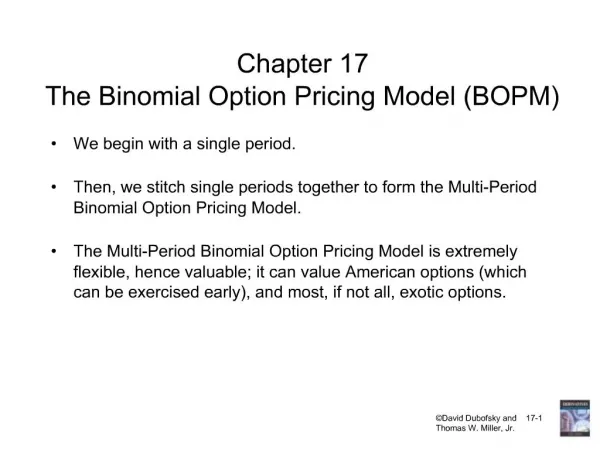
8. The Binomial Model • The first model that we will study is called the Binomial Option Pricing Model (BOPM). • This model assumes that given a value for the stock price, at the end of the next period, the price can either be up by X% or down by Y%.

9. Binomial Model (Cont…) • Since the stock price can take on only one of two possible prices subsequently, the name Binomial is used to describe the process. • We will first study the model using a single time period. • That is, we will assume that we are at time T-1, and that the option will expire at T.

10. The One Period Model • Let the current stock price be S0. • At the end of the period, the price ST can be

11. The One Period Model (Cont…)

12. One Period (Cont…) • Y in this case is obviously a negative number. • The stock price tree may be depicted as follows.

13. The Stock Price Tree

14. Binomial Model (Cont…) • Now consider a European call option. • We will denote the exercise price by E, since X has already been used to denote an up movement for the stock price. • In the case of the Binomial model, we always start with the expiration time of the option, since the payoffs at expiration are readily identifiable.

15. Binomial (Cont…) • We will then work backwards. • Let us denote the call value if the upper stock price is reached by Cu, and the call value if the lower stock price is reached by Cd. • Cu = Max[0, uS0 – E] • Cd = Max[0, dS0 – E]

16. Binomial (Cont…) • Our objective is to find that value of the call option one period earlier, that is right now. • We will denote this unknown value by C0.

17. A Risk-less Portfolio • In order to price the option, we will consider the following investment strategy. • Let us buy  shares of stock and write one call option. • The current value of this portfolio is: • S0 – C0. • The negative sign in front of the option value indicates a short position.

18. Risk-less Portfolio (Cont…) • In the up state, the portfolio will have a value of: uS0 – Cu • In the down state, the portfolio will have a value of: dS0 – Cd • Suppose we were to select  in such a way that the value of this portfolio is the same in both the up as well as the down state?

19. Risk-less Portfolio (Cont…) • Then this portfolio may be said to be risk-less since there are only two possible states of nature in the next period. • So if: uS0 – Cu = dS0 – Cd

20. Risk-less Portfolio (Cont…) •  is known as the hedge ratio. • Since the portfolio is risk-less it must earn the risk-less rate of return. • Let us define r as 1 + risk-less rate. • If so: • uS0 – Cu = dS0 – Cd = (S0 – C0)r

21. Risk-less Portfolio (Cont…) • Substituting for , we get:

22. The Option Premium • Let us denote (r-d)/(u-d) by p. • Therefore, (u-r)/(u-d) = 1-p. • We can then write C0 as:

23. The Option Premium (Cont…) • This is the one period binomial option pricing formula. • p is known as the Risk Neutral probability.

24. Numerical Illustration • Let the current stock price be 100 and the exercise price of a call option be 100. • Let there be a possibility of a 20% up move in the next period and a 20% down move in the next period. • Let the risk-less rate be 5% per period. • Therefore r = 1.05.

25. Illustration (Cont…) • p = (1.05 - .8)/(1.2-.8) = .625 • 1-p = .375 • Cu = Max[0, 120 – 100] = 20 • Cd = Max[0, 80 – 100] = 0 • C0 = .625x20 + .375x0 ------------------------------------ = 11.9048 1.05

26. The Two-Period Situation • Now let us extend the model to a case where there are two periods to expiration. • That is, the option expires at T, whereas we are standing at T-2. • We will denote the current stock price by S0 • The stock price tree can be depicted as follows.

27. The Stock Price Tree uuS0 uS0 S0 udS0 dS0 ddS0 T-2 T-1 T

28. Two Periods (Cont…) • Once again, we know the payoff from the option at expiration. • Let us go back one period, that is to time • T-1. • At this point in time the problem is essentially a one-period problem, to which we have a solution already.

29. Two Periods (Cont…) • Let us denote the option premia corresponding to values of the stock at time T, as Cuu, Cud, and Cdd. • If so, then:

30. Two Periods (Cont…) • Knowing Cu and Cd, we can work backwards to get C0, using an iterative process. • This procedure can be extended to any number of periods.

31. Numerical Illustration • Let the current stock price be 100. • Consider a call option with two periods to expiration and an exercise price of 100. • Assume that given a stock price, the price next period can be 20% more or 20% less. • Let the risk-less rate of interest be 5%. • The stock price tree will look as follows.

32. The Stock Price Tree 144 120 100 96 80 64 T-2 T-1 T

33. Illustration (Cont…) • p = 0.625 and 1-p = .375. • Cuu = Max[0, 144- 100] = 44 • Cud = Max[0, 96-100] = 0 • Cdd = Max[0,64-100] = 0

34. Illustration (Cont…)

35. Impact of Time to Expiration • As you can see, the value of a two period call is greater than that of a one period call. • Obviously, because European call options always have a non-negative time value.

36. Pricing European Puts • We will illustrate the procedure for the one period case. • The procedure is similar to the one used for call options. • It can easily be extended to the multi-period case.

37. European Puts (Cont…) • Assume that we have a stock with a price of S0, which can either go up to uS0 or go down to dS0. • Consider a one-period put option with an exercise price of E. • Pu = Max[0, E – uS0] • Pd = Max[0, E – dS0]

38. European Puts (Cont…) • Using similar arguments, we can show that: and

39. European Puts (Cont…) • p and 1-p, have the same definitions as before.

40. Numerical Illustration • We will use the same data as before. • That is: S0 = E = 100 • u = 1.20; d = 0.80; r = 1.05 • Pu = Max[0, 100 – 120] = 0 • Pd = Max[0,100 – 80] = 20

41. Illustration (Cont…)

42. Extension to the Multiperiod Case • In the case of a call option with N periods left to expiration:

43. Options on Dividend Paying Stocks • Whenever a stock pays dividends, theoretically, the share price should decline by the amount of the dividend. • This feature can be inbuilt into the binomial option pricing model. • It is critical to know as to when exactly the dividend will be paid.

44. Dividends (Cont…) • Let the stock price be 100, and let there be a possibility of a 20% increase or a 20% decline every period. • Let the risk-less rate of return be 5% per period. • Consider a European call option with three periods to expiration.

45. Dividends (Cont…) • The interesting feature is that the stock will pay a dividend of Rs 16 with one period remaining to expiration. • That is, if the option expires at T, then at T-1, the stock will trade ex-dividend. • What this means is that the dividend is paid an instant before the stock trades at T-1.

46. Dividends (Cont…) • In other words, the observable price at T-1, is post-dividend. • The stock price tree may be modeled as follows.

47. The Stock Price Tree 153.6 144 128 102.4 120 96 96 100 80 64 57.6 64 64 80 38.4 T-3 T-1 T T-2

48. Dividends (Cont…) • Notice that because of the dividend, you get additional branches at time T.

49. Dividends (Cont…)

50. Dividends (Cont…) • Using these values, we can work backwards to T-2.