Logistic Regression
Logistic Regression. Biostatistics 510 March 15, 2007 Vanessa Perez. Logistic regression. Most important model for categorical response (y i ) data Categorical response with 2 levels ( binary : 0 and 1) Categorical response with ≥ 3 levels (nominal or ordinal)

Logistic Regression
E N D
Presentation Transcript
Logistic Regression Biostatistics 510 March 15, 2007 Vanessa Perez
Logistic regression • Most important model for categorical response (yi) data • Categorical response with 2 levels (binary: 0 and 1) • Categorical response with ≥ 3 levels (nominal or ordinal) • Predictor variables (xi) can take on any form: binary, categorical, and/or continuous
Logistic Regression Curve 1.0 0.9 0.8 0.7 Probability 0.6 0.5 0.4 0.3 0.2 0.1 0.0 1 2 3 4 5 6 7 8 9 10 11 12 13 14 15 16 17 18 19 20 21 x
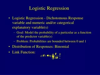
Logit Transformation Logistic regression models transform probabilities called logits. where i indexes all cases (observations). pi is the probability the event (a sale, for example) occurs in the ith case. log is the natural log (to the base e).
Assumption pi (pi )
Logistic regression model with a single continuous predictor logit (pi) = log (odds) = 0 + 1X1 where logit(pi) logit transformation of the probability of the event 0 intercept of the regression line 1 slope of the regression line
LOGISTIC and GENMOD procedure for a single continuous predictor PROC LOGISTIC DATA= dataset <options>; MODEL response=predictor /<options>; OUTPUT OUT=SAS-dataset keyword=name </option>; RUN; PROC GENMOD DATA=dataset <options>; MAKE ‘OBSTATS’ OUT=SAS-data-set; MODEL response=predictors </ options>; RUN;
Descending option in proc logistic and proc genmod • The descending option in SAS causes the levels of your response variable to be sorted from highest to lowest (by default, SAS models the probability of the lower category). • In the binary response setting, we code the event of interest as a ‘1’ and use the descending option to model that probability P(Y = 1 | X = x). • In our SAS example, we’ll see what happens when this option is not used.
Interpretation of a single continuous parameter • The sign (±) of β determines whether the log odds of y is increasing or decreasing for every 1-unit increase in x. • If β > 0, there is an increase in the log odds of y for every 1-unit increase in x. • If β < 0, there is a decrease in the log odds of y for every 1-unit increase in x. • If β = 0 there is no linear relationship between the log odds and x.
Parameter interpretation (ctd). • Exponentiating both sides of the logit link function we get the following: = odds = exp(0 + 1X1) = e 0 e 1X1 • The odds increase multiplicatively by eβfor every 1-unit increase in x. • Whether the increase is greater than 1 or less than one depends on whether β >0 or β <0. • The odds at X = x+1 are eβtimes the odds at X = x. • Therefore, eβis anodds ratio!
Logistic regression model with a single categorical (≥ 2 levels) predictor logit (pi) = log (odds) = 0 + kXk where logit(pi) logit transformation of the probability of the event 0 intercept of the regression line k difference between the logits for category k vs. the reference category
LOGISTIC and GENMOD procedures for a single categorical predictor PROC LOGISTIC DATA=dataset <options>; CLASS variables </option>; MODEL response=predictors </options>; OUTPUT OUT=SAS-data-set keyword=name </option>; RUN; PROC GENMOD DATA=dataset <options>; CLASS variables </option>; MAKE ‘OBSTATS’OUT=SAS-data-set; MODEL response=predictors </ options>; RUN;
Class statement in proc logistic • SAS will create dummy variables for a categorical variable if you tell it to. • We need to specify dummy coding by using the param = ref option in the class statement; we can also specify the comparison group by using the ref = option after the variable name. • Using class automatically generates a test of significance for all parameters associated with the class variable (table of Type 3 tests); if you use dummy variables instead (more on this soon), you will not automatically get an “overall” test for that variable. • We will see this more clearly in the SAS examples.
Reference category • Each factor has as many parameters as categories, but one is redundant, so we need to specify a reference category. • Similar concept to what you just learned for simple linear regression.
Interpretation of a single categorical parameter • If your reference group is level 0, then the coefficient of βk represents the difference in the log odds between level k of your variable and level 0. • Therefore, eβis anodds ratio for category k vs. the reference category of x.
Creating your own dummy variables and not using the class statement • An equivalent model uses dummy variables (that you create), which accounts for redundancy by not including a dummy variable for your reference category. • The choice of reference category is arbitrary. • Remember, this method will not produce an “overall” test of significance for that variable.
Hypothesis testing • Significance tests focuses on a test of H0: β = 0 vs. Ha: β ≠ 0. • The Wald, Likelihood Ratio, and Score test are used (we’ll focus on Wald method) • Wald CI easily obtained, score and LR CI numerically obtained. • For Wald, the 95% CI (on the log odds scale) is
95% CI for parameter • Similarly, the Wald 95% CI for the odds ratio is obtained by exponentiation. • The following yields the lower and upper 95% confidence limits: • 1.96 corresponds to z0.05/2, where z~N(0,1)
Hypothesis testing (ctd) • The Wald statistic of the test H0: β = β0 is • Under H0, the test statistic is asymptotically chi-sq. with 1 df (at α = 0.05, the critical value is 3.84).
References • Paul D. Allison, “Logistic Regression Using the SAS System: Theory and Application”, SAS Institute, Cary, North Carolina, 1999. • Alan Agresti, “Categorical Data Analysis”, 2nd Ed., Wiley Interscience, 2002. • David W. Hosmer and Stanley Lemeshow “Applied Logistic Regression”, Wiley-Interscience, 2nd Edition, 2000.

