Download

1 / 25
290 likes | 815 Vues
Neoclassical Trade Theory: Tools to Be Employed. Appleyard & Field (& Cobb): Chapters 5–7. Basic Concepts for the Consumer Theory. Bundle = combination of goods (that are being consumed)

E N D
Neoclassical Trade Theory: Tools to Be Employed Appleyard & Field (& Cobb): Chapters 5–7
Basic Concepts for the Consumer Theory • Bundle = combination of goods (that are being consumed) • If a consumer gets the same amount of utility from bundle A as from bundle B, she is indifferent between A and B • Indifference curve is a set of all bundles that yield the same utility • Slope of the indifference curve = marginal rate of substitution (MRS) = the increase of one good needed to compensate the loss of another good • diminishing MRS declining marginal utility convex indifference curve concave utility function
Indifference Curve (two goods) Good Y Higher utility 12 Indifference curve 2 4 Indifference curve 1 3 10 Good X
Budget Constraint and the Equilibrium • Budget constraint (budget line) = maximum combinations of goods that can be bought with a fixed level of income (given the prices) • Consumer maximizes her utility given her income and prices consumer chooses the highest indifference curve available • In equilibrium: MRS= MUY/MUX = PX/PY
The Consumer Equilibrium Good Y • Budget Constraint: PX*X+PY*Y= income • Y=income/PY – PX/PY*X That is, slope of the budget constraint = –PX/PY • Indifference Curve: MUX*X+MUY*Y=initial utility • Y = (initial utility)/MUY-MUX/MUY*X That is, slope of the indifference curve = -MUX/MUY Equilibrium: PX/PY=MUX/MUY=MRS y* x* Good X
Marginal Utility & Product • Marginal utility = the additional utility from consuming an additional (very small) unit of a good. • Typically we assume that this is decreasing as consumption of a good increases, e.g. increasing the consumption of water from zero to one litre a day increases utility more than a change of consumption from 1000 to 1001 litre a day. • Marginal product = additional output from using an additional (very small) unit of factor of production. • Typically we assume that if you keep the other factors of production constant, the marginal product is decreasing, e.g. you have 10 shovels (capital), then increasing the number of workers from 9 to 10 increases output more than increasing the workers from 10 to 11.
Production: Capital and Labour Low K/L ratio High K/L ratio Capital (K) Capital (K) Labour (L) Labour (L)
Basic Concepts for the Production Theory • Isoquant = combinations of inputs that produce the same level of output • Slope of the isoquant = Marginal rate of technical substitution (MRTS) = the increase of an input needed to maintain the level of output after a decrease of another input • Isocost = combination of factors that can be bought for given input costs
Producer Equilibrium • Isocost: PK*K+PL*L=cost of production • K=(cost of production)/PK – PL/PK*L Capital • Isoquant: MPPK*K+MPPL*L=output • K = (output)/MPPK-MPPL/MPPK*K Equilibrium: MRTS=MPPL/MPPK=PL/PK (Firm chooses inputs to minimize the cost for given output) K* Isoquant Isocost L* Labour
Generalizing for the Whole Economy • Community Indifference Curve • If a give amount of good X is taken away from the economy how much of good Y is needed to put all consumers back to their initial utility level? • Production Possibilities Frontier • What can be produced given the resources of the economy (≈ budget constraint of the country) • Instead of thinking about individuals, we now use the same ideas to think about whole countries. Note, however, that while this gives us the great gain of being able to use the powerful framework of the decision theory, one should be cautious of thinking about countries as if they were individuals. This point will be discussed in more detail later in the course.
Production Possibilities Frontier (PPF): Constant Opportunity Cost Good Y 40 20 10 20 Good X
PPF: Increasing Opportunity Cost Good Y • Why? • Rising marginal cost • Specific factors • Different factor intensities 40 15 5 10 20 22 Good X
Autarky Equilibrium Good Y Equilibrium: MRT = PX/PY = MRS Y* Community Indifference Curve slope = -MUY/MUX = -MRS Production Possibilities Slope = -PX/PY Slope = -Marginal Rate of Transformation (MRT) X* Good X
Gains from Trade Assuming: • Costless factor mobility • Full employment of factors of production • The indifference curve can show welfare changes For more discussion, see Appleyard and Field around page 93-95. (PX/PY)FT Good Y Equilibrium: MRT = (PX/PY)FT = MRS YC Imports YA YP (PX/PY)A XC XP XA Good X Exports
Consumption and Production Gains (PX/PY)FT Good Y production gain consumption gain (PX/PY)A Good X
Mutual Gains Country 1 Country 2 (PX/PY)FT (PX/PY)FT Good Y Good Y YP Exports YC YA YC Imports YA YP (PX/PY)A (PX/PY)A XC XA XP XP XA XC Good X Good X Exports Imports Note that the graphs are not drawn accurately. In a two-country model, the amount of imports of good Y from Country 1 must equal the amount of exports of good Y to Country 2 (and similarly for good X…)
Identical PPF, Different Preferences (PX/PY)FT Good Y (PX/PY)A (PX/PY)A Good X
Defining Central Concepts for Neoclassical Trade Theory • Terms of Trade = PX/PM • the world price of a country's exports relative to the world price of its imports • PX/PY in the two-country-two-goods-model • terms of trade “improve” when this index rises, i.e. for the same amount of exports the country will get a larger amount of imports • Offer Curve = reciprocal demand curve indicating country’s quantity of imports and exports at all terms of trade
Other Concepts Called “Terms of Trade” • Income Terms of Trade = (PX/PM)*QX • Index of total export earningsPX*QX divided by price of imports country’s ability to import • Single Factoral TOT=(PX/PM)*OX • O=productivity index. Intuition: the amount of imports available for unit of work effort • Double Factoral TOT=(PX/PM)*(OX /OM)
Imports of good Y Exports of good X Note that there is a mistake in A&F Figure 4 page 99 (in the 4th ed.) Deriving the Offer Curve Offer Curve Good Y YC (PX/PY)1 = TOT1 Imports1 YP (PX/PY)2= TOT2 (PX/PY)1 XC XP Good X Exports1 Potential price lines: PX*QX=PY*QY QY=(PX/PY)*QX i.e. given the prices, the value of exports equals the value of imports Good Y YC Imports1 Imports2 YP Imports2 (PX/PY)2 Exports2 XC XP Good X Exports1 Exports2
Offer Curve Offer Curve Offer Curve Imports of good X Imports of good Y Exports of good Y (PX/PY)1 (PX/PY)1 (PX/PY)2 (PX/PY)2 Imports of good X Exports of good X Exports of good Y Putting the Offer Curves to One Graph Country 2 Country 1
Trading Equilibrium:The determination of international prices (PX/PY)E = TOTE (PX/PY)’ Country 2’s offer curve Good Y: Imports to country 1 exports from country 2 Country 1’s offer curve Good X: Exports from country 1 Imports to country 2
Imports of good Y Exports of good X Shift of Offer Curves (1) • Assume that in Country 1 there is shift in preferences and the taste for imports (good Y) increases • That is, for every terms of trade, country 1 is willing to trade more • That is, the offer curve shifts rightwards OC1 OC0 (PX/PY)1 (PX/PY)2
Shift of Offer Curves (2) New equilibrium: • More trade • New terms of trade = new relative prices • (PX/PY)E’ < (PX/PY)E • i.e. the relative price of good Y increase (PX/PY)E = TOTE (PX/PY)E’ = TOTE’ Country 2’s offer curve Good Y: Imports to country 1 exports from country 2 Country 1’s offer curves Good X: Exports from country 1 Imports to country 2
Improvement in Terms of Trade:Substitution, Production and Income Effects • Improvement in Terms of Trade relative price of the exported good X increases relative price of the imported good Y decreases • Substitution effect: consumers shift their purchases towards the imported goods • Production effect: producers start producing more exports • Income effect (terms-of-trade effect): real income of the home country rises (more demand for both X and Y)