Expected Utility Theory

The most famous example of such a theory was published by von Neumann and Morgenstern (1944) (VNM). They proposed it as a “normative” theory of behaviour. That is, classical utility theory as a “normative” theory of behaviour. Classical utility theory was not intended to describe how people actually behave, but how people would behave if they followed certain requirements of rational decision-making. Expected Utility Theory 1 Tuesday, 10 June 20146:21 AM

One of the main purposes of such a theory was to provide an explicit set of assumptions or axioms that underlie rational decision-making. Once VNM specified these axioms, decision researchers were able to compare the mathematical predictions of expected utility theory with the behaviour of real decision makers. When researchers documented violations of an axiom, they often revised the theory and made new predictions. In this way, research on decision making cycled back and forth between theory and observation. Expected Utility Theory 2

What are the axioms of rational decision-making? • Most formulations of expected utility theory are based at least in part on some subset of the following six principles (briefly introduced last week): • 1. Ordering of alternatives. First of all, rational decision makers should be able to compare any two alternatives. They should either prefer one alternative to the other, or they should be indifferent to them. Expected Utility Theory 3

2. Dominance. Rational actors should never adopt strategies that are “dominated” by other strategies (here adopting a strategy is equivalent to making a decision). • A strategy is weakly dominant if, when you compare it to another strategy, it yields a better outcome in at least one respect and is as good or better than the other strategy in all other respects (where “better” means that it leads to an outcome with greater utility). Expected Utility Theory 4

A strategy is strongly dominant if, when you compare it to another strategy, it yields an outcome that is superior in every respect. For example, Car A strongly dominates Car B if it is superior in mileage, cost and looks and is weakly dominant if it gets better mileage than Car B but is equivalent in cost and looks. According to expected utility theory, perfectly rational decision makers should never choose a dominated strategy, even if the strategy is only weakly dominated. Expected Utility Theory 5

3. Cancellation. If two risky alternatives include identical and equally probable outcomes among their possible consequences, then the utility of these outcomes should be ignored in choosing between the two options. • In other words, a choice between two alternatives should depend only on those outcomes that differ, not on outcomes that are the same for both alternatives. Common factors should cancel out. Expected Utility Theory 6

4. Transitivity. If a rational decision maker prefers Outcome A to Outcome B, and Outcome B to Outcome C, then that person should prefer Outcome A to Outcome C. Expected Utility Theory 7

5. Continuity. For any set of outcomes, a decision maker should always prefer a gamble between the best and worst outcomes to a sure intermediate outcome if the odds of the best outcome are good enough. This means, for example, that a rational decision maker should prefer a gamble between £100 and complete financial ruin to a sure gain of £10, provided the odds of financial ruin are one to a googol. Expected Utility Theory 8

6. Behaviour. The Invariance Principle stipulates that a decision maker should not be affected by the way alternatives are presented. For example, a rational decision maker should have no preference between a compound gamble (e.g. a two stage lottery with a fifty percent chance of success on each stage and a £100 payoff if both stages yield successful outcomes) and the simple gamble to which it can be reduced (i.e. a one stage lottery with a twenty five percent chance of winning £100). Expected Utility Theory 9

VNM proved mathematically that when decision makers violate principles such as these, expected utility is not maximised. Expected Utility Theory 10

To take an example, suppose that in violation of the Transitivity Principle, you have intransitive preferences for Outcomes A, B and C. You prefer Outcome A to Outcome B, Outcome B to Outcome C and Outcome C to Outcome A. A►B B►C C►A A►B B►C C►A This means that I should be able to give you Outcome C and offer – say, for a penny – to take back Outcome C and give you Outcome B. Because you prefer Outcome B to Outcome C, you would undoubtedly accept my offer and pay the penny. Expected Utility Theory 11

A►B B►C C►A Now you have Outcome B. In the same way, I should be able to offer – for another penny – to take back Outcome B and give you Outcome A. Because you prefer Outcome A to Outcome B, you would undoubtedly accept my offer and pay the penny. A►B B►C C►A Now you have Outcome A. In the same way, I should be able to offer – for another penny – to take back Outcome A and give you Outcome C. Because you prefer Outcome C to Outcome A, you would undoubtedly accept my offer and pay the penny. Expected Utility Theory 12

The result is that you are back where you started from, with Outcome C, minus three pennies (or £3, or £3000, or …). In other words, I can continue to use this intransitivity in preferences as a “money pump” until your supply of money runs out. Expected Utility Theory 13

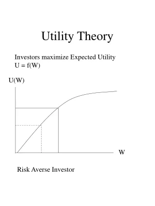
Kahneman and Tversky (1979) argue that utility theory is not an adequate descriptive model and propose an alternative account of choice under risk. In expected utility theory risk aversion is equivalent to the concavity of the utility function. The prevalence of the purchase of insurance against large and small losses has been regarded by many as strong evidence for the concavity of the utility function for money. Expected Utility Theory 14

Why otherwise would people spend so much money to purchase insurance policies at a price that exceeds the expected actuarial cost? However, an examination of the relative attractiveness of various forms of insurance does not support the notion that the utility function for money is concave everywhere. For example, people often prefer insurance programmes that offer limited coverage with low or zero deductible over comparable policies that offer higher maximal coverage with higher deductibles – contrary to risk aversion (Fuchs 1976). Expected Utility Theory 15

As Rabin and Thaler (2001) point out, expected utility theory is used ubiquitously in theoretical and empirical economic research. Despite its central place, however, we will show that this explanation for risk aversion is not plausible in most cases where economists invoke it. Expected Utility Theory 16

To help see why we make such a claim, suppose we know that Johnny is a risk-averse expected utility maximiser, and that he will always turn down the 50‑50 gamble of losing $10 or gaining $11. What else can we say about Johnny? Specifically, can we say anything about bets Johnny will be willing to accept in which there is a 50 percent chance of losing $100 and a 50 percent chance of winning some amount $Y? Expected Utility Theory 17

Consider the following multiple-choice quiz: From the description above, what is the biggest Y such that we know Johnny will turn down a 50-50 lose $100/win $Y bet? a) $110 b) $221 c) $2,000 d) $20,242 e) $1.1 million f) $2.5 billion g) Johnny will reject the bet no matter what Y is. h) We can’t say without more information about Johnny’s utility function Make a note of your choice. Expected Utility Theory 18

You are reminded that we are asking what is the highest value of Y making this statement true for all possible preferences consistent with Johnny being a risk-averse expected utility maximiser who turns down the 50/50 lose $10/gain $11 for all initial wealth levels. You can make no ancillary assumptions, for instance, about the functional form of Johnny’s utility function beyond the fact that it is an increasing and concave function of wealth. Expected Utility Theory 19

Consider the following multiple-choice quiz: From the description above, what is the biggest Y such that we know Johnny will turn down a 50-50 lose $100/win $Y bet? a) $110 b) $221 c) $2,000 d) $20,242 e) $1.1 million f) $2.5 billion g) Johnny will reject the bet no matter what Y is. h) We can’t say without more information about Johnny’s utility function Make a note of your revised choice. Expected Utility Theory 20

Did you guess a, b, or c? If so, you are wrong. Guess again. a) $110 b) $221 c) $2,000 d) $20,242 e) $1.1 million f) $2.5 billion g) Johnny will reject the bet no matter what Y is. h) We can’t say without more information about Johnny’s utility function Expected Utility Theory 21

Did you guess d? Maybe you figured we wouldn’t be asking if the answer weren’t shocking, so you made a ridiculous guess like e, or maybe even f. If so, again you are wrong. Perhaps you guessed h, thinking that the question is impossible to answer with so little to go on. Wrong again. Expected Utility Theory 22

Recall a) $110 b) $221 c) $2,000 d) $20,242 e) $1.1 million f) $2.5 billion g) Johnny will reject the bet no matter what Y is. h) We can’t say without more information about Johnny’s utility function Expected Utility Theory 23

The correct answer is g {Johnny will reject the bet no matter what Y is.}. Johnny will turn down any bet with a 50 percent risk of losing at least $100, no matter how high the upside risk. Johnny would, of course, have to be insane to turn down bets like d, e, and f. So, what is going on here? In conventional expected utility theory, risk aversion comes solely from the concavity of a person’s utility defined over wealth levels. Expected Utility Theory 24

Johnny’s risk aversion over the small bet means, therefore, that his marginal utility for wealth must diminish incredibly rapidly. This means, in turn, that even the chance for staggering gains in wealth provide him with so little marginal utility that he would be unwilling to risk anything significant to get these gains. The problem here is much more general. Expected Utility Theory 25

Using expected utility to explain anything more than economically negligible risk aversion over moderate stakes such as $10, $100, and even $1,000 requires a utility-of-wealth function that predicts absurdly severe risk aversion over very large stakes. Since this theory and its generalisation, the cumulative prospect theory (Tversky and Kahneman 1992) are essentially mathematical theories they will not be further explored here. See case 22 on the module web site. Expected Utility Theory 26

Expected Utility Theory Conventional expected utility theory is simply not a plausible explanation for many instances of risk aversion that economists study. 7.27 27

The following paradox was developed by Allais (1953). Which do you prefer? Allais Paradox Most prefer 1A 28

In notation choosing 1A over 1B because U(1 mill.) > 0.89 U(1 mill.) +0.01 U(0) + 0.1 U(5 mill.) So 0.11 U(1 mill.) > 0.01 U(0) + 0.1 U(5 mill.) Allais Paradox Most prefer 1A 29

The following paradox was developed by Allais (1953). Which do you prefer? Allais Paradox Most prefer 2B 30

In notation choosing 2B over 2A because 0.9 U(0) + 0.1 U(5 mill.) > 0.89 U(0)+ 0.11 U(1 mill.) So 0.01 U(0) + 0.1 U(5 mill.) > 0.11 U(1 mill.) Allais Paradox Most prefer 2B 31

From 1 0.11 U(1 mill.) > 0.01 U(0) + 0.1 U(5 mill.) From 2 0.01 U(0) + 0.1 U(5 mill.) > 0.11 U(1 mill.) Whoops! Allais Paradox 32

Allais Paradox There have been many tests of the descriptive validity of the axioms of expected utility theory using money outcomes. Such tests are relatively uncommon with respect to health outcomes. This is unfortunate, because the standard gamble – considered by many health economists to be the gold standard for cardinal health state value assessment – is implied from the axioms of expected utility. 7.33 33

Allais Paradox The classic Allais paradox, which predicts a systematic violation of the independence axiom, is tested in the context of health outcomes. Seventeen of 38 participants demonstrated strict violations of independence, with 14 of these violating in the direction predicted by Allais. The violations were thus significant and systematic. Moreover, the participants’ qualitative explanations for their behaviour show seemingly rational and not inconsistent reasoning for the violations. This evidence offers a further challenge to the descriptive validity of expected utility (Oliver 2003). 7.34 34

Allais Paradox What appeared to happen is that when the participants were asked to rate an option that gives a positive outcome for certain against an option that has a small probability of immediate death, they often focused upon the small probability of immediate death, which may have induced risk averse behaviour. 7.35 35

Allais Paradox With an identical difference in the percentage chance of immediate death between the two options, but with a large chance of death in both options, the participants often appeared to attach less weight to the probability of death and were more likely to base their preference on the option that gave the best possible outcome, which resulted in seemingly risk seeking behaviour. 7.36 36

Allais Paradox These explanations are consistent with both loss aversion and the over weighting of small probabilities. By increasing the probability of death in both treatment options across contexts, and thus by omitting certainty (and negating the certainty effect), the prominent attribute in the contexts switched, for many participants, from probability to outcome, which appears to explain at least some of the violations of independence (Oliver 2003a). 7.37 37

Expected Utility Theory The study of risky decision making has long used monetary gambles to study choice, but many everyday decisions do not involve the prospect of winning or losing money. Monetary gambles, may be processed and evaluated differently than gambles with nonmonetary outcomes. Whereas monetary gambles involve numeric amounts that can be straightforwardly combined with probabilities to yield at least an approximate “expectation” of value, nonmonetary outcomes are typically not numeric and do not lend themselves to easy combination with the associated probabilities. Compared with monetary gambles, the evaluation of nonmonetary prospects typically proves less sensitive to changes in the probability range, which, among other things, can yield preference reversals (McGraw et al. 2010). 7.38 38

Expected Utility Theory For a list of useful references, see Smith and von Winterfeldt (2004). 7.39 39

Expected Utility Theory Gollier and Muermann (2010) propose a new decision criterion under risk in which individuals extract both utility from anticipatory feelings before the event and disutility from disappointment after the event. They propose a new decision criterion under uncertainty by allowing individuals to extract utility from dreaming about the future and disutility from being disappointed after the event. With such an approach, optimal beliefs balance the benefits of higher expectations against the costs of worse decision making and are necessarily biased toward optimism. They showed that a larger weight on savouring (prior to the event) increases risk aversion and hence reduces the allocation in the risky asset. 7.40 40

Expected Utility Theory This is an alternative to “the classical expected utility model, decision makers are assumed to be stonemen”. In their work they take into account of both anticipatory feelings and disappointment. Disappointment theory was first introduced by Bell (1985). Bell observes that the effect of a salary bonus of $5,000 on the worker’s welfare depends upon whether the worker anticipated no bonus or a bonus of $10,000. Bell (1985) builds a theory of disappointment on this observation, taking the anticipated payoff as external. The new model combines Bell’s (1985) disappointment theory with Akerlof and Dickens’ (1982) notion of anticipatory feelings. 7.41 41

Expected Utility Theory There exists experimental support for the trade-off between optimism and disappointment that underlies the formation of beliefs in the model. Mellers et al. (1997) and Shepperd and McNulty (1998, 2002) provide evidence that people’s feeling about an outcome is determined in part by counterfactual thinking — such as disappointment — which can come from expectations about the future. In an experiment with recreational basketball players, McGraw et al. (2004) show that overconfidence while making shots is negatively correlated with the average pleasure of the outcome. 7.42 42

The Six Laws of Experienced Utility Satisfaction in experiencing the future depends on decisions made today. Baucells and Sarin (2013) consider six well-known psychological laws governing satisfaction – “The Six Laws of Experienced Utility”. A very brief summary is given here, see the original paper for an extensive bibliography and much more mathematical detail. 7.43 43

The Six Laws of Experienced Utility 1 Relative Comparison - The first law states that experienced utility is determined by reality minus expectations. Frijda (1988) calls relative comparison the law of change. Kahneman and Tversky (1979) and Tversky and Kahneman (1991) demonstrate that the carrier of utility is the change from a reference level and not the final outcome. 7.44 44

The Six Laws of Experienced Utility 2 Motion of Expectations - The second law of experienced utility asserts that expectations change. Three factors affect expectations. First, expectations can be a function of the consumption of our peer group (social comparison). Second, expectations can be a function of our past consumption (adaptation). Third, expectations can be changed by seeing reality in a new way (reframing). 7.45 45

The Six Laws of Experienced Utility 3 Aversion to Loss - The third law of experienced utility says that losses are felt more keenly than equivalent gains. 7.46 46

The Six Laws of Experienced Utility 4 Diminishing Sensitivity - Experienced utility is not proportional to the difference between consumption and the habituation level; rather, the increase in experienced utility slows as consumption moves further from the habituation level. This implies that each additional unit of consumption gives a smaller increment of satisfaction. Simply put, this law states that experienced utility cannot be easily taken to blissful or tragic extremes. The increase in experienced utility slows as reality moves further from the reference point. It is well known in psychophysics that doubling the stimulus does not always double the intensity of the response. 7.47 47

The Six Laws of Experienced Utility 5 Satiation - Satiation is one of the lingering effects that recent consumption has on current consumption. Recent consumption reduces the experienced utility of subsequent consumption, and recent abstinence increases the experienced utility of subsequent consumption. 7.48 48

The Six Laws of Experienced Utility 6 Projection - People forecast that future preferences and feelings will be more similar to their current preferences and feelings than they actually will be. This implies that when we predict the satisfaction of future consumption, our prediction is not very different from the satisfaction we would experience if we were to realize this consumption now. For example, shoppers who are hungry overbuy food because when they are in a hungry state, food—even if it is for future consumption—seems more attractive. 7.49 49

The Six Laws of Experienced Utility Similarly, they may choose a variety of snacks today for consumption in future periods. Projecting today’s static preferences, the same snack over and over seems very satiating, and the way to counteract this is by choosing a high level of variety. But satiation wanes with the passage of time, and when the choice is made sequentially, consumers may stick with the same snack. 7.50 50

Expected Utility Theory