Utility Theory
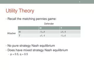
Utility Theory. Recall the matching pennies game: No pure strategy Nash equilibrium Does have mixed strategy Nash equilibrium p = 0.5, q = 0.5. Defender. Attacker. Utility Theory. Consider a modification to the matching pennies game: What is the mixed strategy Nash equilibrium?. Defender.

Utility Theory
E N D
Presentation Transcript
Utility Theory • Recall the matching pennies game: • No pure strategy Nash equilibrium • Does have mixed strategy Nash equilibrium • p = 0.5, q = 0.5 Defender Attacker
Utility Theory • Consider a modification to the matching pennies game: • What is the mixed strategy Nash equilibrium? Defender Attacker
Utility Theory • Consider a modification to the matching pennies game: • What is the mixed strategy Nash equilibrium? • Still p = 0.5, q = 0.5 Defender Attacker
Utility Theory • A further modification: • What is the mixed strategy Nash equilibrium? Defender Attacker
Utility Theory • A further modification: • What is the mixed strategy Nash equilibrium? • Still p = 0.5, q = 0.5 Defender Attacker
Utility Theory • Another modification: • What is the mixed strategy Nash equilibrium? Defender Attacker
Utility Theory • Another modification: • What is the mixed strategy Nash equilibrium? • Still p = 0.5, q = 0.5! Defender Attacker
Utility Theory • Another modification: • What is the mixed strategy Nash equilibrium? • Still p = 0.5, q = 0.5! • What if this were in $1000’s? • What would you do if you were the attacker? • Would you still play heads with 0.5 probability? Defender Attacker
Utility Theory • Utility is a measure of total worth of an outcome • Takes more into account than just payoff; decision maker’s attitude toward risk can be considered as well • Payoffs are assigned utilities, depending on how useful or desirable they are to a decision maker • Often uses a 0-1 scale, where the least desirable outcome has a utility of 0 and the most desirable outcome has a utility of 1. Other scales such as 0-10 and 0-100 are also used • Applicable in economic theory, game theory and decision theory
Lotteries • Consider a decision problem with 3 possible outcomes: • A: $400,000 • B: -$100,000 • C: $100,000 • The decision maker has a choice between two alternatives; • 1) Take a 50-50 chance on receiving either -$100,000 or $400,000 • 2) Receiving $100,000 for certain • Expected Payoff for each alternative: • 1) $150,000 • 2) $100,000
Simple Lotteries • Choice 1 is a lottery between either losing $100,000 or receiving $400,000 • With expected payoff of $150,000 • Choice 2 can be thought of as a lottery with a single outcome ($100,000) • These are examples of simple lotteries, where the chance event leads to immediate payoffs 0.5 0.5 1 100,000 -100,000 400,000
Compound Lotteries • The outcomes of a lottery can themselves be further lotteries. These are referred to as compound lotteries • Compound lotteries can always be reduced to simple lotteries 0.3 0.4 0.4 0.6 0.3 400,000 100,000 -100,000 100,000 0.5 0.5 400,000 -100,000
Preferences • Let A and B be alternatives • Choices, outcomes, strategies, etc • Anything that one needs to choose among • Let ≻, ≽ and ~ denote: • A ≻ B: “A is preferred over B” • A ≽B: “A is preferred at least as much as B” • A ~ B: “A and B are equally preferable”
Von Neumann-Morgenstern Theory of Utility • John von Neumann and Oskar Morgenstern, 1947 • Developed as a component of game theory • Four axioms of rationality: • Completeness • Transitivity • Independence • Continuity
Axiom 1: Completeness • Completeness assumes that an individual has well defined preferences and can always decide between any two alternatives. • Axiom (Completeness): For every A and B either A ≽ B orB ≽ A. • This means that the individual either prefers A to B, or is indifferent between A and B, or prefers B to A.
Axiom 2: Transitivity • Transitivity assumes that, as an individual decides according to the completeness axiom, the individual also decides consistently. • Axiom (Transitivity): For every A, B and C with A ≽ B and B ≽ C, we must have A ≽ C.
Axiom 3: Independence • Independence also pertains to well-defined preferences and assumes that two gambles mixed with a third one maintain the same preference order as when the two are presented independently of the third one. The independence axiom is the most controversial one (see Allais’ paradox) • Independence of irrelevant alternatives assumes that a preference holds independently of the possibility of another outcome: • Axiom (Independence): Let A, B, and C be three lotteries with A ≻ B, and let t be a value in (0,1]; then • tA+ (1-t)C ≻ tB + (1-t)C.
Axiom 3: Independence • Example: • If L1a is preferred, then L1b should be preferred L1a: L2a: 1 0.5 0.5 400,000 -100,000 100,000 L2b: 0.1 L1b: 0.1 0.9 0.45 0.45 500,000 -100,000 400,000 500,000 100,000
Axiom 4: Continuity • Continuity assumes that when there are three lotteries (A, B and C) and the individual prefers A to B and B to C, then there should be a possible combination of A and C in which the individual is then indifferent between this mix and the lottery B. • Axiom (Continuity): Let A, B and C be lotteries with A ≽ B ≽ C; then there exists a probability p such that B is equally as good as pA + (1-p)C.
VNM Theory of Utility • For any decision-maker satisfying the four axioms of rationality, there exists a utility function u such that • A ≻ B iff u(A) > u(B) • VNM Theory of Expected Utility • Let A and B be lotteries • Then A ≻ B iffE(u(A)) > E(u(B)) (or rewritten as Eu(A) > Eu(B)) where • For lottery A with outcomes A1, A2, … An, each occurring with probability p1, p2,… pn, • Eu(A) = p1*u(A1) + p2*u(A2) + … + pn*u(An) • Similarly for B
Result • Any agent acting to maximize the expectation of a function u will obey axioms 1–4 • Thus expected utility maximization results in rational decision-making • Recall that game theory depends on rational choice
Determining Utilities • Returning the original choice over two lotteries • Which would you prefer? • The less risky alternative (L1) • The one with higher payoff (L2) • VNM theory of expected utility tells us that • L1 ≻ L2 implies that Eu(L1) > Eu(L2) 0.5 0.5 1 L1: L2: 100,000 -100,000 400,000
Determining Utilities • Since L1 = $100,000, Eu(L1) = u(100,000) • Thus u(100,000) > Eu(L2) • u(100,000) > 0.5u(-100,000) + 0.5u(400,000) • If we enforce u(L) in [0,1] for all alternatives L • And let -100,000 and 400,000 be the worst and best possible outcomes, respectively, in the decision problem, then: • u(-100,000) = 0 • u(400,000) = 1 • So u(100,000) > 0.5(0) + 0.5(1) = 0.5
Determining Utilities • What does this tell us? • Not much, yet • What if we changed the probabilities of the lottery to make it more enticing: • Perhaps in this case the lottery would be preferred 0.3 0.7 1 L1: L2: 100,000 -100,000 400,000
Determining Utilities • Change the lottery probabilities again, making it slightly less attractive • If the decision-maker becomes indifferent between the two alternatives, then • u(100,000) = 0.4(0) + 0.6(1) = 0.6 • And the outcome 100,000 is said to be the certainty equivalent of lottery L2 0.4 0.6 1 L1: L2: 100,000 -100,000 400,000
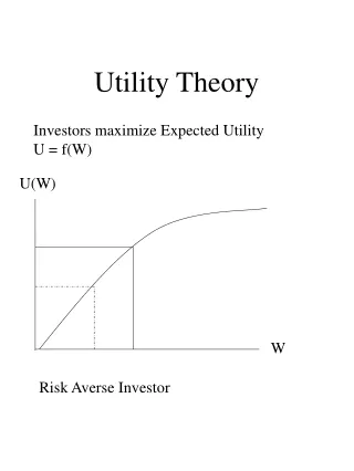
Risk Aversion • A utility function u is said to be risk-averse if, for any lottery L with expected payoff p • Eu(L) < u(p) • In other words, the decision maker will always prefer the expected payoff for certain over a gamble with equivalent expectation • Similarly a risk-averse utility function will make the certainty equivalent of a lottery lower than it’s expectation • E.g. For L2 with expected payoff $200,000, u’s certainty equivalent was $100,000
Law of Diminishing Marginal Utility • From economics • The marginal utility of a good or service is defined as the gain from an increase or loss from a decrease in the consumption of that good or service • Law of diminishing marginal utility: • Phenomenon that the first unit of consumption of a good or service yields more utility than the second and subsequent units, with a continuing reduction for greater amount • E.g. happiness from having no money and getting $1000 is much greater than our happiness would be if we already had $1,000,000
Other Risk Profiles • A utility function u is said to be risk-seekingif, for any lottery L with expected payoff p • Eu(L) > u(p) • A utility function u is said to be risk-neutralif, for any lottery L with expected payoff p • Eu(L) = u(p)
Back to the Original Problem • What if this were in $1000’s? • What would you do if you were the attacker? • Would you still play heads with 0.5 probability? Defender Attacker
Back to the Original Problem • What if this were in $1000’s? • What would you do if you were the attacker? • Would you still play heads with 0.5 probability? • Tendency to prefer H might display risk-averse behaviour • Need to compute utility to properly assess payoffs Defender Attacker
Utility Assessment • Suppose A is indifferent between: • A lottery where he receives • 0 with 0.4 probability • 200 with 0.6 probability • 100 for certain • If 0 and 200 are the worst and best outcomes, respectively, then • u(100) = 0.4(0) + 0.6(1) = 0.6
Payoff Matrix with Utilities • We can then rewrite the payoff matrix: • Where each players’ utilities are known to both players (an assumption of mixed strategy Nash equilibria) • Then the new mixed strategy Nash equilibria is? Defender Attacker
Payoff Matrix with Utilities • We can then rewrite the payoff matrix: • Where each players’ utilities are known to both players (an assumption of mixed strategy Nash equilibria) • Then the new mixed strategy Nash equilibrium is? • p = 0.5, q = 0.6 Defender Attacker