Ordinal Utility and Demand Theory-I
110 likes | 558 Vues
Ordinal Utility and Demand Theory-I. Introduction. We know that the Marshallian Demand curve is based upon the assumptions that: (1) The utilities derived from consuming n-commodities are independent and are additive . (4.1)……………… and (2) The level of utility is cardinally measurable.

Ordinal Utility and Demand Theory-I
E N D
Presentation Transcript
Introduction • We know that the Marshallian Demand curve is based upon the assumptions that: • (1) The utilities derived from consuming n-commodities are independent and are additive . • (4.1)……………… • and (2) The level of utility is cardinally measurable. • However, to many economists, these assumptions are unjustified and unnecessary.
Because, plausibly, a utility function should be a joint function of all consumed as: • U=φ(x1,x2,………,xn) (4.2) • Assume this utility function possesses continuous first and second derivatives with respect to all its variables, φij is less than or greater than 0, i≠j, indicating the MU derived from xi is not independent of xj. • A meaningful demand function for a commodity can be derived under a less restrictive assumption, namely when utility is merely ordinal.
Demand Theory Based upon Utility Function • Properties of Utility Function: Let us assume X1 and X2 are two goods consumed. • For a given time period, the consumer’s tastes are fixed which can be represented by the utility function • U=φ(x1,x2), where x1 and x2 > 0 (4.3) • The utility function φ(x1,x2), where x1,x2> 0 possesses continuous first and second derivatives with respect to x1 and x2. • The economic meaning of these derivatives of U are as follows:.
i) The term φ1 and φ2 denote MU1(=dU/dx1) and MU2(=dU/dx2), where MU1 and MU2 > 0 (4.2) • The term φ11 (φ22) denotes the rate of change in MU of X1 (X2) due to a Δ in the quantity of X1 (X2) consumed. φ11 , φ22 may be less than, equal to or greater than 0. • The term φ21 (φ12) denotes the rate of change in MU of X2 (X1) due to a Δ in the quantity of X1 (X2) consumed. φ12 , φ21 may be less than, equal to or greater than 0. • φ12 = φ21→ that the effect of a Δ in the quantity of X1 consumed on the MU of X2 is the same as the effect of a Δ in the quantity of X2 consumed on the MU of X1.
The Consumer Equilibrium • The consumer will purchase, under a given income constraint, that combination of goods which will give him/her the highest level of utility/satisfaction. • For any given time period the consumer’s tastes are represented by U=φ(x1,x2), where x1 and x2 > 0. • We also assume that the consumer’s money income is fixed, say at M0. If we also assume that the prices of X1 and X2 are P1 and P2, which are constant, The consumer budget constraint is represented by equation: • P1x1 + P2 x2=M0. (4.4)
The Consumer Equilibrium • Maximizing U=φ(x1,x2), subject to budget constraint (4.4) is equivalent to maximizing the following Lagrangean function wrt to x1 and x2 where • The FOC for maximization the consumer utility is maximized when • Or • Or • and P1x1 + P2 x2=M0 …….(4.8)
The Consumer Equilibrium • The MRS21 = (dx2/dx1). According to (4.3) to substitute X2 for X1 and to keep the consumer’s total utility at a constant level, implies that φ1dx1+φ2dx2 = 0. • However, this equation implies that • (dx2/dx1) = - (φ1/φ2). • The term - (φ1/φ2) also represent the MRS21. • The eq (4.7) states that the consumer utility in maximized when the MRS21 = negative of the price ratio of P1 to P2, subject to the budget constraint. • The eq.4.8 states that the consumer is at equilibrium when the last penny spent on X1 and X2 yield the same amount of MU, subject to the budget constraint.
The Consumer Equilibrium • The Lagrangean multiplier λ, at equilibrium, can be shown to be the MU of money. • From the utility function U=φ(x1,x2) we know that • (i) dU = φ1dx1+φ2dx2 (ii) φ1= λP1 and φ2= λP2 • Substituting (ii) into (i) we obtain (iii) dU = λ(P1dx1+P2dx2). • However, from eq. 4.4 assuming P1 and P2 are constants and M a variable, we know that (iv) P1dx1+P2dx2=dM • Substituting (iv) into (iii) we obtain (v) λ= (dU/dM), thus λ is the MU of money.
Demand Functions and Demand Curves • Solving the FOC (4.6) simultaneously we may derive the following demand functions: • x1 = f1 (P1, P2, M), x1 > 0, and x2 = f2 (P2, P1, M), x2 > 0 • The demand curves for X1 and X2 are respectively given by • x1 = f1 (P1; P02, M0), x1 > 0, and x2 = f2 (P2; P01, M0), x2 > 0