Utility theory
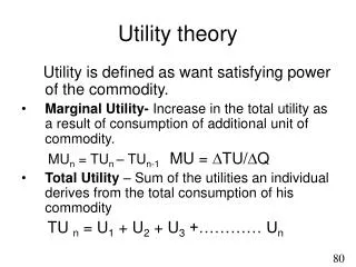
Utility theory. Utility is defined as want satisfying power of the commodity. Marginal Utility- Increase in the total utility as a result of consumption of additional unit of commodity. MU n = TU n – TU n-1 MU = TU/ Q

Utility theory
E N D
Presentation Transcript
Utility theory Utility is defined as want satisfying power of the commodity. • Marginal Utility- Increase in the total utility as a result of consumption of additional unit of commodity. MUn = TUn – TUn-1 MU = TU/Q • Total Utility – Sum of the utilities an individual derives from the total consumption of his commodity TU n = U1 + U2 + U3 +………… Un 80
Approaches to measurement of utility- • Cardinal Utility approach • Ordinal Utility approach • Indifference Curve Approach • Revealed Preference Hypothesis 81
CARDINAL UTILITY APPROACH • Utility can be measured in monetary units by the amount of money consumer is ready to sacrifice for another unit of commodity. • Measurement of utility can be done in subjective unit called utils 82
ORDINAL UTILITY APPROACH • The utility is not measurable. • Consumer should be able to determine the order of preferences among different bundle of goods. • Consumer need not know in specific units the utility of various commodity to know his preferences. 83
CARDINAL - Assumptions • Rationality • Cardinal Utility • Diminishing Marginal Utility • Constant Utility of Money • Utility is additive 84
Consumer Equilibrium • When a consumer pays price for the commodity he is consuming, he compares the utility he derives from the additional unit of commodity with the utility he sacrifices in terms of price paid for the unit of commodity MU = P In case there are more than two commodities the equilibrium condition may be expresses as 85
Criticism of Cardinal Approach • Satisfaction derived from various commodities cannot be measured objectively • Money used for measurement is not correct as it is not constant and the value of money keeps fluctuating. • It is psychological concept, therefore the very law is questionable. • The cardinal approach considers the effect of price changes on the demand curve ( price effect). This assumption is unrealistic as the price effect may include income and substitution effect 87
Ordinal Utility Approach- assumptions • Rationality • Utility is Ordinal • Diminishing Marginal Rate of Substitution • The total utility of the consumer depends on the quantity of the commodity consumed i.e. U=f (q1 q2 ….qn) • Consistency and transitivity of choice • Non satiety 88
Indifference Curve An indifference curve may be defined as the locus of points giving particular combination or bundle of goods which yield the same utility or level of satisfaction to the consumer so that he is indifferent as to the particular combination he consumes. 89
Indifference Curve Map • A number of indifference curves representing various levels if satisfaction form an indifference map 91
Properties of Indifference Curve • Indifference curve have negative slope • Indifference Curve are Convex to Origin • Indifference cannot touch or Intersect each other • Higher Level of Indifference Curve Represents Higher Level of Satisfaction 92
DIFFERENT SHAPE OF INDIFFERENCE CURVE Perfect Substitutes Perfect Complimentary 93
Consumer Equilibrium • Budget Constraint-Income acts as a constraint in the attempt for maximizing utility and is known as budget constraint. Y = px qx+ py q y 94
Two conditions must be fulfilled for the consumer to be in equilibrium • Scope of Indifference Curve (MRS) should be equal to the slope of budget line • At the point of consumer equilibrium, indifference curve is convex to the origin, i.e. MRS is diminishing 97
Derivation of Demand Curve Using IC Approach P Budget lineshifts New Equilibrium (E2) Point of Tangency of BLS & Higher IC (Price Consumption Curve) Join successive points On QY axis to get DD 98
Derivation of Demand Curve Using IC Approach Change in the consumption basket as a result of Changes in price is called price effect. The total price effect comprises of two components (a) substitution effect (b) income Effect 99
When the price of a commodity changes, the price of the substitute remaining the same, the price ratio changes (given constant money income). The change in the relative price induces substitution of cheaper good for the expensive one. This change is referred to a substitution effect. • If the price of a commodity decreases, the consumer’s real income increases. The change in the consumption basket due to change in the real income in called income effect 100
There are two methods followed for splitting the total price effect into income effect and substitution effect. • Hicksian approach • Slutsky approach Hicks assumes constancy of real purchasing power of the consumer by keeping the consumer on the same satisfaction level. Slutsky keeps real purchasing power constant in the sense that the consumer could purchase the original combination of commodities. 101
Slutsky Approach – Income & Substitution Effect (Price Fall) 104
STATISTICAL METHOD BAROMETRIC METHOD ECONOMETRIC METHODS TREND PROJECTION LEAD INDICATORS GRAPHICAL METHOD REGRESSION METHODS COINCIDENTAL INDICATORS TREND FITTING / LEAST SQUARE METHODS SIMULTANEOUS EQUATIONS LAG INDICATORS BOX-JENKINS METHOD
FITTING TREND EQUATION 1. Linear Trend S=a+bT 2. Exponential Trend Y = a ebT Log Y = Log a + bT
S=a+bT ∑S=na +b∑T ∑ST=a∑T + b∑T2 See table 1, 164=10a+55b 1024=55a+385b , by solving these two equations we get the trend equation as S=8.26+1.48T For 11th year S = 8.26+ 1.48 (11) = 24,540 tonnes
BOX JENKINS METHOD • Used for short term projection • Uses stationary time series data Steps in Box Jenkins Method 1.Eliminate trend from time series data 2.Make sure there is seasonality in stationary time series data (if value of one or more coefficients are different from zero, it reveals seasonality in time series data) 3. Apply models to it.
(1)Auto-regressive model Yt = a1Yt-1 + a2Yt-2 +…..+anYt-n + et et is random portion of Y which is not explained by the model (2) Moving Average model Yt = m + b1et-1 + b2et-2 +….+bpet-p + et (3) Auto regressive moving average model Yt = a1Yt-1 + a2Yt-2+..+anYt-n+b1et-1+b2et-2+…+ bpet-p + et
Simple Regression Method Y = a + bX ∑Y = na + b∑X ∑XY = ∑Xa + b∑X2 See table 490 = 7a +152 b 12,000= 152a+ 3994b By solvingthese equation we get Y = 27.44 + 1.96 X
Multi- variate method QX = a - bPx +cY +dPy+jA Simultaneous Equation Model Yt = Ct + It +Gt + Xt Ct = a + bYt