Utility Theory in Decision-Making
Learn about utility theory in making decisions involving risk and uncertainty with monetary values. Explore attitudes towards risk and how utility values help determine preferences. Understand expected value and utility functions.

Utility Theory in Decision-Making
E N D
Presentation Transcript
Option 1: • bet that pays $5,000,000 if a coin flipped comes up tails • you get $0 if the coin comes up heads. Option 2: get $2,000,000 with certainty Expected Marginal Value of the two options: 1. EMV of the bet = .5(5,000,000) + .5(0) = 2,500,000 2. EMV sure deal = 1(2,000,000) = 2,000,000 Choosing the option with the highest EMV has been our decision rule. But with a sure bet we may decide to avoid the risky alternative. Would you take a sure $2,000,000 over a risky $5,000,000?
In general we say people have one of three attitudes toward risk. People can be risk avoiders, risk seekers (or risk lover) , or indifferent toward risk (risk neutral). Utility Value Risk neutral Risk avoider Risk lover Monetary Value Utility values are assigned to monetary values and the general shape for each type of person is shown above. Note that for equal increments in dollar value the utility either rises at a decreasing rate (avoider), constant rate or increasing rate.
Once you have the utility values associated with the money values if you graph them out you can see what type of person you have: risk avoider, lover of a person indifferent to risk. What I do in the rest of this section is expand your “feel” for this method. You can probably stop here to work on problems, but I carry on if you need that feel.
Say we have an opportunity that is uncertain. We could get 50000 p percent of the time, but we could get -50000 (1-p) percent of the time. The expected value of the uncertain opportunity is defined as p(50000) + (1-p)(-50000). Once we have a value for p we could calculate the expected value. As an example, say p = .3. Then the expected value is .3(50000) + .7(-50000) = -20000. Now, let’s think about the three types of people again. Say each has to compare an opportunity with a certain -20000 with the uncertain opportunity I just mentioned.
On the next slide I show the utility function for each type of person. Note at -20000 I have a higher number assigned (by height of curve) for risk avoider, then neutral, then lover. Note the number just represents preference or utility for a person. Higher numbers for a person means higher utility for that person. But, we can not compare numbers across people and say because one has a higher number than another that one prefers it more than another. We will not compare across people.
Here we show a generic example with a risk avoider. Two monetary values of interest are, say, X1 and X2 and those values have utility U(X1) and U(X2), respectively Utility U(X2) U(X1) $ X1 X2
Say the outcome of a risky decision is to have X1 occur p% of the time and X2 occur (1 – p)% . Then the EMV is p(X1) + (1 – p)(X2). The expected utility of the risky decision is found in a similar way and without proof I tell you the expected utility is Utility U(X2) U(X1) EU $ EMV X1 X2 along the straight line connecting the points on the curve directly above the EMV for the decision. We have the expected utility as EU = pU(X1) + (1 – p)U(X2)
Remember the uncertain option had possible outcomes 50000 or -50000 and an expected value = -20000 (because we had p = .3). The certain option was to get -20000 (lose 20000) a b c Monetary Value -50 -30 -20 0 20 30 50 For the certain option the utility is just read off the utility function or curve for each person. The values are represented by letters a, b, and c for the risk avoider, neutral, and lover types, respectively.
Example States of Nature Alternatives s1 s2 s3 d1 30000 20000 -50000 d2 50000 -20000 -30000 d3 0 0 0 Also say P(s1) = .3, P(s2) = .5, and P(s3) = .2. Next we will go through a process used to assign utility values to each value in the payoff table. In general we will say U(x) is the utility value assigned to the payoff value x. Note that 50000 is the highest payoff and -50000 is the lowest payoff in this problem.
Let’s assign the number 10 as the utility for the highest payout, 50000. Thus U(50000) = 10. Let’s assign 0 as the utility for the lowest payout, -50000. So, U(-50000) = 0. We could have used other numbers to represent the utility, but the main point is higher payouts get higher utility numbers. Next, we will consider a method to assign utility values to all the other payoff values in the table. First consider a lottery. Say that there is probability p that if the lottery is played the manager will win 50000 (the highest value in the payoff table), and there is a (1-p) probability the manager will win -50000 (the lowest value in the payoff table). The lottery has an expected utility pU(50000) + (1-p)U(-50000) = p(10) + (1-p)0 = p(10).
Remember the expected utility is on a straight line between the uncertain points on the utility function. The straight line would be the utility function for the risk neutral person. The curved line shown is for a risk avoider. The straight line is also the expected utility line for the risk avoider. Utility is 10 here Utility is zero here -50 -30 -20 20 30 50
Next we have to assign utility values to each of the other payoff values in the table. Let’s start with the value 30000. We will assume for a short time that 30000 can be had with certainty. If p, the probability of getting the 50000 in the lottery, is 1 or close to 1, then the person is very likely to get the 50000 and thus the lottery is likely to be preferred to the certain 30000. But if p is close to 0 the person is likely to get -50000 and thus the certain 30000 would be preferred. There is a value of p such that the person would have an equal preference for the lottery and the certain 30000. The individual would then be said to be indifferent between the lottery and the certain value. p is then called the indifference probability.
The 30000 is the certain deal. For the risk avoider the utility of 30000 is on the curve above 30000. The expected value of the lottery is p(50000) + (1-p)(-50000) = p100000 – 50000. This expected value would equal 30000 if p = .8 Let’s look at the expected utility of the lottery again. We had p10. If p = .8 the expected utility of the lottery would be 8 and this would be the height of the straight line above 30000. So, the utility curve above 30000 has to be assigned a value above 8 if the person is risk averse or is a risk avoider. There is some value for p above .8, but less than 1 that would make the lottery equally attractive as the certain 30000. This probability is called the indifference probability. In the real world the decision maker has to grapple with what this value is. We will take it as a given piece of information.
For the certain value 30000, say the indifference probability is .95. With p = .95 the expected utility of the uncertain option is .95(10) + .5(0) = 9.5 and since the utility of the certain option is the same, U(30000) = 9.5 Similarly, say for all the other values in our payoff table we get the indifference probabilities as seen in the table below and the associated utility values. Payoff value indiff. Prob utility 30000 .95 9.5 20000 .90 9.0 0 .75 7.5 -20000 .55 5.5 -30000 .4 4.0
So, we take the original payoff table States of Nature Alternatives s1 s2 s3 d1 30000 20000 -50000 d2 50000 -20000 -30000 d3 0 0 0 And change all the values to utility values States of Nature Alternatives s1 s2 s3 d1 9.5 9. 0 d2 10 5.5 4.0 d3 7.5 7.5 7.5 We had P(s1) = .3, P(s2) = .5, and P(s3) = .2. Next we calculate the expected utility of each option. The calculation is similar to the expected value calculation.
The expected utility for each is d1 .3(9.5) + .5(9.0) + .2(0) = 7.35 d2 .3(10) + .5(5.5) + .2(4.0) = 6.55 d3 .3(7.5) + .5(7.5) + .2(7.5) = 7.5 Option 3 has the best expected utility, so we choose option 3.