Mean-Variance as Expected Utility
Mean-Variance as Expected Utility. Lecture 4. Expected Utility IV(1). Expected Utility/Expected Value-Variance. Expected Utility IV(2). Expected Utility IV(3). Next, we want to complete the square in the exponent. Expected Utility IV(4). Elicitation of Risk Aversion Coefficients

Mean-Variance as Expected Utility
E N D
Presentation Transcript
Mean-Variance as Expected Utility Lecture 4
Expected Utility IV(1) • Expected Utility/Expected Value-Variance
Expected Utility IV(3) • Next, we want to complete the square in the exponent
Expected Utility IV(4) • Elicitation of Risk Aversion Coefficients • Equally Likely Certainty Equivalence (ELCE) • Experience has shown that manipulation of probabilities while holding the consequences fixed is not very satisfactory. • Thus, most methods involve changing the monetary gamble while keeping the probabilities fixed. • One way to do this is to hold the gamble at 50/50 or make the outcomes equally likely.
Expected Utility IV(5) • In this method you cut a gamble by eliciting the decision maker’s certainty equivalence.
Expected Utility IV(6) • Equally Likely but Risky Outcomes (ELRO) method is similar, but instead of varying the certainty equivalence, you form two lotteries and vary one of the payoffs until the decision maker is indifferent between the two lotteries.
Expected Utility IV(7) • Other transformations of the Arrow-Pratt risk aversion coefficient. • Following Raskin and Cochran, we turn to the use of published risk aversion coefficients. • Rederiving the Arrow-Pratt measures
Expected Utility IV(9) • This association between the risk aversion and the level of income then raises the question of the change in outcome scale. • For example, what if the original utility function was elicited on a per acre basis, and you want to use the results for a whole farm exercise? • Theorem 1: Let r(x)=u’’(x)/u’(x). Define a transformation of scale on x such that w=x/c, where c is a constant. Then r(w)=cr(x).
Expected Utility IV(11) • Theorem 2: If v=x + c, where c is a constant, then r(v)=r(x). Therefore, the magnitude of the risk aversion coefficient is unaffected by the use of incremental rather absolute returns. • Example: Suppose that a study of U.S. farmers gives a risk aversion coefficient of r=.0001/$ (U.S.) Application to the Australian farmers whose dollar is worth .667 of the U.S. dollar is r=.0000667/$ Australian