Univariate Regression Variance, Slope & Correlation
230 likes | 1.14k Vues
Univariate Regression Variance, Slope & Correlation. MSIT3000 Lecture 18. Objectives. Learn how to estimate the disturbance in a regression model. Assess the usefulness of an OLS model through the slope: using hypothesis tests, and confidence intervals

Univariate Regression Variance, Slope & Correlation
E N D
Presentation Transcript
Univariate RegressionVariance, Slope & Correlation MSIT3000 Lecture 18
Objectives • Learn how to estimate the disturbance in a regression model. • Assess the usefulness of an OLS model through the slope: • using hypothesis tests, and • confidence intervals • Compare correlation & covariance to OLS. Text: Chapter 9, sections 4 through 7; 2.9 & 2.10.
Estimating Var() = 2 • We use the observed error term (e) to estimate the disturbance [or predicted error term] (). • s2 = SSE/(n-2) • Remember, SSE = (y-yhat)2 • We divide by n-2 because that is how many degrees of freedom left after we estimated the intercept and the slope.
Interpreting s2 • Use the Empirical rule. We would expect “most” observations of y to be within two standard deviations (2s) of our prediction (yhat). • s = s2 has several names. The text calls it “the estimated standard error of the regression model”. SAS calls it Root MSE (for Mean Squared Error); see the SAS output on p 498. s2 is called “the estimated variance”.
When does the slope tell us anything at all ? • The model is: • Y = 0 + 1*X + • If X has no impact on Y, the slope must be zero.
How can we test whether or not the model is useful? • We perform a hypothesis test to find out if the data suggest the slope is NOT equal to zero. • This is the default output from most statistical software. • What do we need to know in order to perform this Hypothesis Test? • The distribution of the slope-estimate under the null hypothesis.
The distribution of 1-hat • If we know the variance of the disturbance, the variance of the slope is: • Var(1-hat) = ²/SS(xx) • In that case, the distribution of 1–hat would be: • 1-hat ~ N(1, /[SS(xx)] )
The distribution of 1-hat (realistically) • When we don’t know the standard error, we have to estimate the standard deviation of the disturbance using s: • s² = SSE/(n-2) s = (SSE/[n-2]) • And our test statistic is t distributed • just like our small sample tests for means.
Testing whether X impacts Y: • We want the burden of proof on the model, so the hypotheses are: • H0: 1 = 0 • H1: 1 0 • The second step is to find the rejection region (RR): • Our test statistic is t-distributed with n-2 degrees of freedom, therefore: • RR = < - , - t/2 ] [t/2 , >
Testing whether X impacts Y continued: • Step III: Calculate the test statistic. • TS = (1-hat – 0)/S 1-hat • Remember, under the null hypothesis, 1 = 0. If you wished to test the null hypothesis that • 1 = 1 you would subtract 1 in the numerator above. • You divide by the standard deviation of 1-hat: • S 1-hat = S/[SS(xx)] • where S2 = SSE/[n-2] • Step IV: Conclude.
P-values and Confidence Intervals • When you perform a hypothesis test you can also calculate the p-value, just as you would for a small-sample HT for a mean. • And you can also create a Confidence Interval (CI): • CI = 1-hat ± t/2 * S1-hat
Objective 3: Alternative measures of linear relationship • We will now consider: • Covariance • Correlation • The Coefficient of Determination
Covariance • Covariance measures how much to variables “move around together”:
Covariance Matrix This is extremely useful in presenting how stocks relate to one another!
The Correlation Coefficient • The Pearson moment coefficient of correlation • (or simply the “correlation coefficient”): • r = SS(xy)/[SS(xx)*SS(yy)] • -1 r 1 • Note that b1 has the same numerator [i.e. SS(xy)], so if the slope is zero, the correlation coefficient is also zero. • r is an estimator for the linear correlation between x and y in the population: • [rho]
Correlation Coefficient and Covariance • These two measure the same thing, but correlation is bound between –1 and 1:
The Coefficient of Determination • The Coefficient of Determination is a measure of how much of the variation in y is explained by x. • The Coefficient of Determination will be useful also when we have multiple x’s to explain y. This is not true of the correlation coefficient.
If x explained nothing... • ...what would be the relationship between SS(yy) and SSE? • SS(yy) = ( y – ybar )² • SSE = ( y – yhat )²
If x explained nothing... • ...what would be the relationship between SS(yy) and SSE? • SS(yy) = ( y – ybar )² • SSE = ( y – yhat )² • If x explains nothing, the best predictor for y, regardless of the value of x, would be ybar. • Therefore, if x explains nothing, we would expect: • SS(yy) = SSE • and if x explains very little, we would expect SS(yy)SSE.
A measure of how much x explains: • Out of the total variation in y [SS(yy)], a measure of how much x explains is: • SS(yy) – SSE [this is explained variation] • But because this does not have a useful scale, we calculate the proportion explained: • r² = [SS(yy) – SSE]/SS(yy) • r² = 1 – [SSE/SS(yy)] • Note: 0 r² 1
Conclusion • Objectives addressed: • Learn how to estimate the error in a regression model. • Assess the usefulness of an OLS model through the slope: • using hypothesis tests, and • confidence intervals • Compare correlation & covariance to OLS. • Problems: • Text: 9.24; 9.31a, 9.34, 9.39, (9.54) • Exam 3A, 7-9 & 17-21.