Download
1 / 41
410 likes | 568 Vues
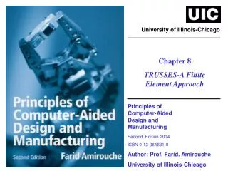
University of Illinois-Chicago. Chapter 7 Introduction to Finite Element Method. Principles of Computer-Aided Design and Manufacturing Second Edition 2004 ISBN 0-13-064631-8 Author: Prof. Farid. Amirouche University of Illinois-Chicago. CHAPTER 7. 7.1 Introduction.

E N D
University of Illinois-Chicago Chapter 7 Introduction to Finite Element Method Principles of Computer-Aided Design and Manufacturing Second Edition 2004 ISBN 0-13-064631-8 Author: Prof. Farid. Amirouche University of Illinois-Chicago
CHAPTER 7 7.1 Introduction 7.1 INTRODUCTION FEM is a technique that discretizes a given physical or mathematical problem into smaller fundamental parts, called ‘elements’ . Then an analysis of the element is conducted using the required mathematics. Figure 7.1 A finite element mesh of hip prosthesis Principles of Computer-Aided Design and Manufacturing Second Edition 2004 – ISBN 0-13-064631-8 Author: Prof. Farid. Amirouche, University of Illinois-Chicago
CHAPTER 7 7.1 Introduction Figure 7.2 A output of stress distribution after simulation Principles of Computer-Aided Design and Manufacturing Second Edition 2004 – ISBN 0-13-064631-8 Author: Prof. Farid. Amirouche, University of Illinois-Chicago
CHAPTER 7 7.2 Basic Concepts in FEM 7.2BASIC CONCEPTS IN THE FINITE-ELEMENT METHOD The basic steps in FEA (Finite Element Analysis) consists of 3 phases: • Preprocessing Phase: • 1) Create and discretize the solution domain into finite elements; that is ,subdivide the problem into nodes and elements. • 2) Assume a shape function to represent the physical behavior of an element; that is, an approximate continuous function • is assumed to represent the solution of an element. • 3) Develop equations for an element. • 4) Assemble the elements to present the entire problem. Construct the global stiffness matrix. • 5) Apply boundary conditions, initial conditions, and loading. Principles of Computer-Aided Design and Manufacturing Second Edition 2004 – ISBN 0-13-064631-8 Author: Prof. Farid. Amirouche, University of Illinois-Chicago
CHAPTER 7 7.2 Basic Concepts in FEM b) Solution Phase 6) Solve a set of linear or nonlinear algebraic equations simultaneously to obtain nodal results, such as displacement values at different nodes or temperature values at different nodes in a heat transfer problem. c) Post processor Phase 7) Obtain other important information. At this point, you may be interested in values of principal stresses, heat fluxes, etc. Principles of Computer-Aided Design and Manufacturing Second Edition 2004 – ISBN 0-13-064631-8 Author: Prof. Farid. Amirouche, University of Illinois-Chicago
CHAPTER 7 7.2 Basic Concepts in FEM Figure 7.3 A general discretization of a body into finite elements Principles of Computer-Aided Design and Manufacturing Second Edition 2004 – ISBN 0-13-064631-8 Author: Prof. Farid. Amirouche, University of Illinois-Chicago
CHAPTER 7 7.2 Basic Concepts in FEM where ke (e being the element) is the local element stiffness matrix, fe is the external forces applied at each element, uerepresents the nodal displacements for the element, and feadd represents the additional forces.(7.1) Assuming Equation 7.1 reduces to (7.2) In terms of stresses and strains equation (7.2) becomes e = seue (7.3) where eis the element stress matrix, and se is the constitutive relationship connecting ue and e . Principles of Computer-Aided Design and Manufacturing Second Edition 2004 – ISBN 0-13-064631-8 Author: Prof. Farid. Amirouche, University of Illinois-Chicago
CHAPTER 7 7.2 Basic Concepts in FEM Example 7.1 A load of P =180 lbs act on the variable cross sectional bar in which one end is fixed and a compressive load act at the other end. Dimensions of the bar are shown in the figure 7.4. Calculate the deflection at various points along its length. Calculate the reaction force at the fixed end and compute stresses in each element. Figure 7.4(a) A variable cross-sectional bar subject to a compressive load Principles of Computer-Aided Design and Manufacturing Second Edition 2004 – ISBN 0-13-064631-8 Author: Prof. Farid. Amirouche, University of Illinois-Chicago
CHAPTER 7 7.2 Basic Concepts in FEM Solution : From figure 7.4 we compute the cross-sectional areas , and assign values of the Young’s modulus of elasticity to each of the segment bars. A1=2.3248 in2. E1=669400.12 lb/in2 . A2=0.7750 in2. E2=458 lb/in2 . A3=2.0922 in2. E3=669400.12 lb/in2 . P = 180 lb. The stiffness of each bar segment is derived from Hooke’s Law where (7.4) (7.5) (7.6) Principles of Computer-Aided Design and Manufacturing Second Edition 2004 – ISBN 0-13-064631-8 Author: Prof. Farid. Amirouche, University of Illinois-Chicago
CHAPTER 7 7.2 Basic Concepts in FEM Figure 7.4(b) Free body diagram of the forces Principles of Computer-Aided Design and Manufacturing Second Edition 2004 – ISBN 0-13-064631-8 Author: Prof. Farid. Amirouche, University of Illinois-Chicago
CHAPTER 7 7.2 Basic Concepts in FEM Applying the I law of mechanics where F=0, at each node At node 1 (7.7) At node 2 (7.8) At node 3 (7.9) At node 4 (7.10) The above equations can be written in matrix form as (7.11) Principles of Computer-Aided Design and Manufacturing Second Edition 2004 – ISBN 0-13-064631-8 Author: Prof. Farid. Amirouche, University of Illinois-Chicago
CHAPTER 7 7.2 Basic Concepts in FEM Since u1 = 0 , this is equivalent to eliminating row 1 and column 4 of the stiffness matrix. Column 1 The matrix equation (7.11) reduces to (7.12) Plugging in the values for all the Ks and substituting the value of P : (7.13) Principles of Computer-Aided Design and Manufacturing Second Edition 2004 – ISBN 0-13-064631-8 Author: Prof. Farid. Amirouche, University of Illinois-Chicago
CHAPTER 7 7.2 Basic Concepts in FEM From the Equation (7.13) we get: Principles of Computer-Aided Design and Manufacturing Second Edition 2004 – ISBN 0-13-064631-8 Author: Prof. Farid. Amirouche, University of Illinois-Chicago
CHAPTER 7 7.2 Basic Concepts in FEM Example 7.2 This is a similar example to 7.1, however element z is replaced with two identical supports which forms element 2 and 3. A load of P = 180 lbs acts on the variable cross sectional bar in which one end is fixed and a compressive load acts at the other end. Dimensions of the bar are indicated in the figure 7.5. Calculate the deflection at various points along its length. Calculate the reaction force at the fixed end and the corresponding stresses in each element. Figure 7.6 A variable cross-section bar with identical supports in the middle. Principles of Computer-Aided Design and Manufacturing Second Edition 2004 – ISBN 0-13-064631-8 Author: Prof. Farid. Amirouche, University of Illinois-Chicago
CHAPTER 7 7.2 Basic Concepts in FEM The cross sectional areas are found to be The Young’s modulus of elasticity for each segment The load P is: The element stiffness is found as: Principles of Computer-Aided Design and Manufacturing Second Edition 2004 – ISBN 0-13-064631-8 Author: Prof. Farid. Amirouche, University of Illinois-Chicago
CHAPTER 7 7.2 Basic Concepts in FEM At node 1 (7.14) At node 2 (7.15) At node 3 (7.16) At node 4 (7.17) The above equations can be written in matrix form as (7.18) Principles of Computer-Aided Design and Manufacturing Second Edition 2004 – ISBN 0-13-064631-8 Author: Prof. Farid. Amirouche, University of Illinois-Chicago
CHAPTER 7 7.2 Basic Concepts in FEM Since u1 = 0, Equation ( 7.18 ) can be reduced to: (7.19) Substituting the values of Ks and P we obtain The solution of which is found to be Principles of Computer-Aided Design and Manufacturing Second Edition 2004 – ISBN 0-13-064631-8 Author: Prof. Farid. Amirouche, University of Illinois-Chicago
CHAPTER 7 7.2 Basic Concepts in FEM Stresses for each element are obtained as: lb/in2 lb/in2 lb/in2 Principles of Computer-Aided Design and Manufacturing Second Edition 2004 – ISBN 0-13-064631-8 Author: Prof. Farid. Amirouche, University of Illinois-Chicago
CHAPTER 7 7.2 Basic Concepts in FEM Example 7.3 A tapering round bar is fixed at one end and a tensile load P=180 lbs is applied at the other end. The maximum and minimum radius of the bar is 20 in and 10 in respectively. The bar’s modulus of elasticity E = 669400.12 lb/in2. Consider the bar as a set of 4 elements of equal length and uniformly increasing diameter. Find the global stiffness matrix and displacements at each node and reaction force. Figure 7.6 A Tapered round bar subject to a tensile load P Principles of Computer-Aided Design and Manufacturing Second Edition 2004 – ISBN 0-13-064631-8 Author: Prof. Farid. Amirouche, University of Illinois-Chicago
CHAPTER 7 7.2 Basic Concepts in FEM Figure 7.7 A four element representation of the tapered round bar Principles of Computer-Aided Design and Manufacturing Second Edition 2004 – ISBN 0-13-064631-8 Author: Prof. Farid. Amirouche, University of Illinois-Chicago
CHAPTER 7 7.2 Basic Concepts in FEM The geometrical data and stiffness properties for each element are: Since F=0 at each node therefore, (7.20) At node 1 (7.21) At node 2 (7.22) At node 3 (7.23) At node 4 (7.24) At node 5 (7.25) Principles of Computer-Aided Design and Manufacturing Second Edition 2004 – ISBN 0-13-064631-8 Author: Prof. Farid. Amirouche, University of Illinois-Chicago
CHAPTER 7 7.2 Basic Concepts in FEM Applying the boundary conditions, that is u5 = 0 we get (7.26) A solution of which is found to be (7.27) The reaction force is obtained by writing the equation form, (7.25) where (7.28) Substituting the values of u5 and u4 and k4, we obtain (7.29) Principles of Computer-Aided Design and Manufacturing Second Edition 2004 – ISBN 0-13-064631-8 Author: Prof. Farid. Amirouche, University of Illinois-Chicago
CHAPTER 7 7.3 Potential Energy Formulation 7.3 POTENTIAL ENERGY FORMULATION • Finite element method is based on the minimization of the total potential energy formulation. • When close form solution is not possible approximation methods such as Finite Element are the most commonly used in solid mechanics. • To illustrate how finite element is formulated, we will consider an elastic body such as the one shown in Figure 7.9 where the body is subjected to a loading force which causes it to deform. Principles of Computer-Aided Design and Manufacturing Second Edition 2004 – ISBN 0-13-064631-8 Author: Prof. Farid. Amirouche, University of Illinois-Chicago
CHAPTER 7 7.3 Potential Energy Formulation Figure 7.9 Elastic body Principles of Computer-Aided Design and Manufacturing Second Edition 2004 – ISBN 0-13-064631-8 Author: Prof. Farid. Amirouche, University of Illinois-Chicago
CHAPTER 7 7.3 Potential Energy Formulation From Hooke’s Law, we write (7.30) where F represents the compressive force A represents area of the elastic body E represents the young’s modulus of elasticity be the displacement in the y-direction, and L is the length of the segment. From Hooke’s Law the force displacement relationship is where represents the energy (7.32) Principles of Computer-Aided Design and Manufacturing Second Edition 2004 – ISBN 0-13-064631-8 Author: Prof. Farid. Amirouche, University of Illinois-Chicago
CHAPTER 7 7.3 Potential Energy Formulation We can express the energy equation in terms of the stress-strain as: Where represents the element strain energy and the volume of element is we can then write the strain energy for an element introducing the superscript e (7.35) The stress can be substituted for by (7.36) Using the above relation in Equation (7.32 ), we obtain (7.37) Principles of Computer-Aided Design and Manufacturing Second Edition 2004 – ISBN 0-13-064631-8 Author: Prof. Farid. Amirouche, University of Illinois-Chicago
CHAPTER 7 7.3 Potential Energy Formulation The total energy, which consists of the strain energy due to deformation of the body and the work performed by the external forces can be expressed as function of combined energy as Where denotes displacement along the force direction Fi . (7.38) It follows that a stable system requires that the potential energy be minimum at equilibrium (7.39) We know that strain is defined making use of the relative displacement between adjacent elements (7.40) Principles of Computer-Aided Design and Manufacturing Second Edition 2004 – ISBN 0-13-064631-8 Author: Prof. Farid. Amirouche, University of Illinois-Chicago
CHAPTER 7 7.3 Potential Energy Formulation Equation (7.39) has two components. Expression for the first term is (7.41) and (7.42) In matrix form (7.43) where Principles of Computer-Aided Design and Manufacturing Second Edition 2004 – ISBN 0-13-064631-8 Author: Prof. Farid. Amirouche, University of Illinois-Chicago
CHAPTER 7 7.3 Potential Energy Formulation Similarly , we take the second term in (7.39) (7.44) and (7.45) Combining Equations (7.43),(7.44), and (7.45) leads to elemental force-displacement relation (7.46) (7.47) or where k(e) is the element stiffness matrix, u(e) the element displacement associated with node i or i+1 , and F(e) denotes the external forces acting at the nodes. Principles of Computer-Aided Design and Manufacturing Second Edition 2004 – ISBN 0-13-064631-8 Author: Prof. Farid. Amirouche, University of Illinois-Chicago
CHAPTER 7 7.4 Closed Loop Formulation 7.4 CLOSED FORM SOLUTION • The closed form solution is used when all the variables • have explicit mathematical forms that can be dealt with • in terms of extracting a solution. • Consider a continuous body subject to a compressive • load P (Figure 7.10).The objective is to determine the • displacement or deformation at any point. • Let the continuous body have a variable cross-sectional area . Principles of Computer-Aided Design and Manufacturing Second Edition 2004 – ISBN 0-13-064631-8 Author: Prof. Farid. Amirouche, University of Illinois-Chicago
CHAPTER 7 7.4 Closed Loop Formulation Figure 7.9 A non-uniform bar subjected to compressive load P. Principles of Computer-Aided Design and Manufacturing Second Edition 2004 – ISBN 0-13-064631-8 Author: Prof. Farid. Amirouche, University of Illinois-Chicago
CHAPTER 7 7.4 Closed Loop Formulation The equilibrium equation at any cross sectional area cab be written as where (7.48) (7.49) Substituting the above equation into (7.48) we get (7.50) Recall that strain is defined as (7.51) Substituting the above equation into (7.50) we get (7.52) (7.53) Principles of Computer-Aided Design and Manufacturing Second Edition 2004 – ISBN 0-13-064631-8 Author: Prof. Farid. Amirouche, University of Illinois-Chicago
CHAPTER 7 7.4 Closed Loop Formulation Integrating the above equation will lead to exact solution of displacement. (7.54) If we assume the load is constant and that (7.55) Equation (7.48) becomes ( 7.54 ) (7.56) or (7.57) where (7.58) Principles of Computer-Aided Design and Manufacturing Second Edition 2004 – ISBN 0-13-064631-8 Author: Prof. Farid. Amirouche, University of Illinois-Chicago
CHAPTER 7 7.4 Closed Loop Formulation Let Hence, (7.59) , then Let (7.60) or (7.61) Principles of Computer-Aided Design and Manufacturing Second Edition 2004 – ISBN 0-13-064631-8 Author: Prof. Farid. Amirouche, University of Illinois-Chicago
CHAPTER 7 7.4 Closed Loop Formulation The above solution can be used to find displacement at various points Along the length . From (7.58) we have And the displacement is (7.62) and Thus, the solution depends upon which we should know first hand. Principles of Computer-Aided Design and Manufacturing Second Edition 2004 – ISBN 0-13-064631-8 Author: Prof. Farid. Amirouche, University of Illinois-Chicago
CHAPTER 7 7.5 Weighted Residual Method 7.5 WEIGHTED RESIDUAL METHOD • The WRM assumes an approximate solution to the governing differential equations. • The solution criterion is one where the boundary conditions and initial conditions of the problem are satisfied. • It is evident that the approximate solution leads to some marginal errors. • If we require that the errors vanish over a given interval or at some given points then we will force the approximate solution to converge to an accurate solution. Principles of Computer-Aided Design and Manufacturing Second Edition 2004 – ISBN 0-13-064631-8 Author: Prof. Farid. Amirouche, University of Illinois-Chicago
CHAPTER 7 7.5 Weighted Residual Method Consider the differential equation discussed in previous example where (7.63) Let us choose a displacement field u to approximate the solution, that is let (7.64) are unknown coefficients where if we substitute u(y) & A(y) into the differential equation we get (7.65) stands for residual. where Principles of Computer-Aided Design and Manufacturing Second Edition 2004 – ISBN 0-13-064631-8 Author: Prof. Farid. Amirouche, University of Illinois-Chicago
CHAPTER 7 7.5 Weighted Residual Method The equation above has two constants C1 & C2. If we require that εvanishes at two points we will get two equation which can be used to solve for C1 & C2. Solving Equation (7.66) for these conditions , we get (7.65) and (7.66) for The final solution for the displacement field is (7.67) Principles of Computer-Aided Design and Manufacturing Second Edition 2004 – ISBN 0-13-064631-8 Author: Prof. Farid. Amirouche, University of Illinois-Chicago
CHAPTER 7 7.6 Galerkin Method 7.6 GALERKIN METHOD The Galerkin method requires the integer of the error function over some selected interval to be forced to zero and that the error be orthogonal to some weighting functions i, according to the integral (7.68) Where = [ 0 , L ] for i = 1,….., n. i s are selected as part of the approximate solution. This is simply done by assigning the function to the terms to multiply the coefficients. Because we assume as defined in (7.63) then 1= y and 2 = y2. (7.64) Now we use (7.67) and substitute 1= y and the residual ε from (7.65). Furthermore let the values of r1 and r2 be given from Example 7.3 then we obtain, Principles of Computer-Aided Design and Manufacturing Second Edition 2004 – ISBN 0-13-064631-8 Author: Prof. Farid. Amirouche, University of Illinois-Chicago
CHAPTER 7 7.6 Galerkin Method (7.69) P = 180 lb from Example 7.3 (7.70) Solving the above two equations we get & C1y+C2y2 (7.71) The solution is then approximated by Principles of Computer-Aided Design and Manufacturing Second Edition 2004 – ISBN 0-13-064631-8 Author: Prof. Farid. Amirouche, University of Illinois-Chicago
CHAPTER 7 7.6 Galerkin Method Table 7.1 Comparison of displacement values by different methods Principles of Computer-Aided Design and Manufacturing Second Edition 2004 – ISBN 0-13-064631-8 Author: Prof. Farid. Amirouche, University of Illinois-Chicago