Running Time: Estimation Rules
Learn the rules for estimating running time in algorithm analysis, including the most significant term, constants of proportionality, and growth rates. Understand the concepts of "Big-Oh" notation and the asymptotic behavior of algorithms.

Running Time: Estimation Rules
E N D
Presentation Transcript
Running Time: Estimation Rules • Running time is proportional to the most significant term in T(n) • Once a problem size becomes large, the most significant term is that which has the largest power of n • This term increases faster than other terms which reduce in significance COMPSCI.220.S1.T - 2004
Running Time: Estimation Rules • Running time T(n) = 0.25n2+0.5n 0.25n2 COMPSCI.220.S1.T - 2004
Running Time: Estimation Rules • Constants of proportionality depend on the compiler, language, computer, etc. • It is useful to ignore the constants when analysing algorithms. • Constants of proportionality are reduced by using faster hardware or minimising time spent on the “inner loop” • But this would not effect behaviour of an algorithm for a large problem! COMPSCI.220.S1.T - 2004
Algorithm Versus Implementation • Analysis of time complexity takes no account of the constant of proportionality c • Analysis involves relative changes of running time COMPSCI.220.S1.T - 2004
Elementary Operations • Basic arithmetic operations (+ ; – ; ;; % ) • Relational operators ( ==, !=, >, <, >=, <= ) • Boolean operations (AND,OR,NOT), • Branch operations, … Input for problem domains (meaning of n): Sorting: n items Graph / path: n vertices / edges Image processing: n pixelsText processing: string length COMPSCI.220.S1.T - 2004
“Big-Oh” Tool O(…) for Analysing Algorithms Typical curves of time complexity: T(n) log n, T(n) n T(n) n log n T(n) nk T(n) 2n COMPSCI.220.S1.T - 2004
Relative growth: G(n) = f(n)/f(5) COMPSCI.220.S1.T - 2004
“Big-Oh” O(…): Linear Complexity Linear complexity time T(n) n O(n) running time does not grow faster than a linear function of the problem size n COMPSCI.220.S1.T - 2004
Logarithmic “Big-Oh” Complexity Logarithmic complexity: time T(n) log n O(log n) running time does not grow faster than a log function of the problem size n COMPSCI.220.S1.T - 2004
g(n) is O(f(n)), or g(n) = O(f(n)) Function g(n) is “Big-Oh” of f(n) if, starting from some n>n0, there always exist a function c·f(n) that grows faster than the function g(n) COMPSCI.220.S1.T - 2004
“Big-Oh” O(…) : Formal Definition for those who are not afraid of Maths: • Let f(n) and g(n) be positive-valued functions defined on the positive integers n • The function g is defined as O(f) and is said to be of the order of f(n) iff (read: if and only if) there are a real constant c > 0 and an integer n0 such that g(n) c·f(n) for all n>n0 COMPSCI.220.S1.T - 2004
“Big-Oh” O(…) : Informal Meaning for those who are afraid of Maths:g is O(f) means that the algorithm with time complexity g runs (for large n) at most as fast, within a constant factor, as the algorithm with time complexity f Note that the formal definition of “Big-Oh” differs slightly from the Stage I calculus: COMPSCI.220.S1.T - 2004
“Big-Oh” O(…) : Informal Meaning • g is O(f)means that the order of time complexity of the function g is asymptoticallyless than or equal to the order of time complexity of the function f • Asymptotical behaviour only for the large values of n • Two functions are of the same order when they each are “Big-Oh” of the other: f = O(g) AND g = O(f) • This property is called “Big-Theta”: g = Q(f) COMPSCI.220.S1.T - 2004
O(…) Comparisons: Two Crucial Ideas • The exact running time function is not important, since it can be multiplied by any arbitrary positive constant. • Two functions are compared only asymtotically, for large n, and not near the origin • If the constants involved are very large, then the asymptotical behaviour is of no practical interest! COMPSCI.220.S1.T - 2004
“Big-Oh” Examples - 1 Linear function g(n) = an + b; a > 0, is O(n): g(n) < (a + |b|) ·n for all n 1 Do not writeO(2n)orO(an + b)as this means stillO(n)! O(n) - running time: T(n) = 3n + 1 T(n) = 108 + n T(n) = 50 + 10– 8 · n T(n) = 106· n + 1 Remember that “Big-Oh” describes an “asymptotic behaviour” for large problem sizes COMPSCI.220.S1.T - 2004
“Big-Oh” Examples - 2 Polynomial Pk(n) = ak nk + a k-1nk-1 + … + a1n + a0; ak > 0,is O(nk) Do not writeO(Pk(n))as this means stillO(nk)! O(nk) - running time: • T(n) = 3n2+ 5n+ 1 is O(n2) Is it also O(n3)? • T(n) = 10-8n3+ 108n2+ 30 is O(n3) • T(n) = 10-8n8+ 1000n+ 1 is O(n8) COMPSCI.220.S1.T - 2004
“Big-Oh” Examples - 3 Exponential g(n) = 2n+k is O( 2n): 2n+k = 2k · 2n for all n Exponential g(n) = mn+k is O( ln),l m > 1: mn+k ln+k= lk · ln for all n, k • Remember that a “brute-force” search for the best combination of n interdependent binary decisions by exhausting all the 2n possible combinations has the exponential time complexity, and try to find more efficient ways to solve your problem if n 20 … 30 COMPSCI.220.S1.T - 2004
“Big-Oh” Examples - 4 Logarithmic function g(n) = logm n is of order log2 n because logmn = logm 2 · log2n for all n,m > 0 Do not writeO(logmn)as thismeans stillO(log n)! You will find later that the most efficientsearch for data in an ordered array has the logarithmic complexity COMPSCI.220.S1.T - 2004