Download
1 / 15
150 likes | 292 Vues
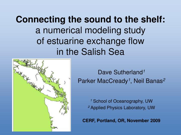
Connecting the sound to the shelf: a numerical modeling study of estuarine exchange flow in the Salish Sea. Dave Sutherland 1 Parker MacCready 1 , Neil Banas 2 1 School of Oceanography, UW 2 Applied Physics Laboratory, UW CERF, Portland, OR, November 2009.

E N D
Connecting the sound to the shelf: a numerical modeling study of estuarine exchange flow in the Salish Sea Dave Sutherland1 Parker MacCready1, Neil Banas2 1School of Oceanography, UW 2 Applied Physics Laboratory, UW CERF, Portland, OR, November 2009
Connecting the sound to the shelf: a numerical modeling study of estuarine exchange flowin the Salish Sea PRISM Acknowledgments: PRISM (Jeff Richey) Barb Hickey, Amy MacFadyen, David Darr (UW) WA DOE All data sources Puget Sound Regional Synthesis Model
The Salish Sea Vancouver Island Strait of Georgia Strait of Juan de Fuca 400 m Puget Sound coastal WA, OR Columbia River
The Straits Salinity, July Salinity, July (Collias et al., 1974) (Masson and Cummins, 2000) • Strait of Juan de Fuca • 100 km long, 20 km wide, 200 m deep • ~0.2 Sv exchange flow • significant spring/neap variability, • seasonal variability, and tidal rectification • (see Martin and MacCready, 2009) • Strait of Georgia • Fraser River: mean ~7500 m3/s, large • seasonal variability • intense mixing in SJI’s and sill regions, • more stratified in basins • significant spring/neap variability
Puget Sound Deception Pass Whidbey Basin Skagit 2 largest rivers (~75% of Puget Sound mean ~1000 m3/s) Snohomish Admiralty Inlet Hood Canal Main Basin South Sound 5 km Tacoma Narrows
Puget Sound exchange flow (cm/s) Main Basin 150 m Salinity, July • Puget Sound • series of reaches (basins) connected by shallow sills • 0.04 Sv exchange flow • ~1000 m3/s river input • large seasonal and spring/neap variability • residence times: range from 5-70 days Hood Canal
river river sill (Ebbesmeyer and Barnes, 1980; Cokelet and Stewart, 1985) Hypothesis: Puget Sound, SJdF, and the SoG are characterized by quiescent reaches (e.g. Main Basin) and turbulent sill regions (e.g. AInlet) Tool: realistic ROMS numerical model setup of the Salish Sea to investigate patterns of exchange flow on varied time and space scales • Construct realistic hindcast simulations for 1998-2008 in Puget Sound and greater Salish Sea region • Puget Sound resolution ~200 m • coastal resolution ~2 km • use best available forcing (rivers, meteorological, boundary)
Model Set-up • Parameters • stretched, spherical grid with 25 vertical • levels, qb = 0.6 and qs = 5 • k-e version of GLS turbulence closure • horizontal diffusivity = 0.5 m2 s-1 • quadratic bottom friction, Cd = 0.003 • hmin = 4 m, rmax ~ 0.7, no wet/dry • Forcing • Boundaries • - Radiation and nudging at southern • and western boundaries (NCOM-CCS) • Atmosphere • - Bulk fluxes from hourly fields from the • MM5 regional forecast model • Rivers • - 19 rivers, daily time series (USGS) • Tides • - 8 constituents calculated from TPXO7.1 • global tide model
Model validation CTD profiles JEMS SJDF ROMS OBS mid Strait of Georgia Whidbey Basin Mooring time-series outside Columbia
Patterns of exchange flow SoG-N AI-N “out-estuary” SoG-mid JdF-W SoG-S WB JdF-mid JdF-E AI-N,S MB “in-estuary” HC (May-July mean) SS |Ue| ~ 20,000 m3/s net Ue ~ 500 m3/s
Patterns of exchange flow SoG-N AI-N “out-estuary” AI-S SoG-mid JdF-W SoG-S WB JdF-mid JdF-E AI-N,S MB “in-estuary” HC (May-July mean) SS
Patterns of exchange flow SoG-N MB-N “out-estuary” MB-mid SoG-mid MB-S JdF-W SoG-S WB JdF-mid JdF-E AI-N,S MB “in-estuary” HC (May-July mean) SS
SoG Patterns of exchange flow JdF AI Strait of Juan de Fuca Strait of Georgia Admiralty Inlet “out estuary” “out estuary” “out estuary” SOG-N JdF-E AI-N SOG-mid JdF-mid AI-S SOG-S JdF-W “in-estuary” “in-estuary” “in-estuary” |Ue| ~ 130,000 m3/s net Ue ~ 6000 m3/s |Ue| ~ 80,000 m3/s net Ue ~ 5000 m3/s |Ue| ~ 20,000 m3/s net Ue ~ 500 m3/s
Variability of exchange flow at Adm. Inlet Skagit Snohomish river discharge (m3/s) N/S winds (m/s) depth mean current (m/s) exchange flow (1000 m3/s) “out-estuary” “in-estuary”
Conclusions • Development underway of realistic, high resolution simulations of Puget Sound and the surrounding coastal ocean • Patterns of exchange flow are useful in characterizing estuarine regions in the Salish Sea and will lead to quantitative comparisons in the future (http://faculty.washington.edu/dsuth/MoSSea/)