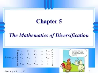
Chapter 5 The Mathematics of Diversification
520 likes | 1.16k Vues
Chapter 5 The Mathematics of Diversification. Introduction. The reason for portfolio theory mathematics: To show why diversification is a good idea To show why diversification makes sense logically. Introduction (cont ’ d). Harry Markowitz ’ s efficient portfolios :

Chapter 5 The Mathematics of Diversification
E N D
Presentation Transcript
Introduction • The reason for portfolio theory mathematics: • To show why diversification is a good idea • To show why diversification makes sense logically
Introduction (cont’d) • Harry Markowitz’s efficient portfolios: • Those portfolios providing the maximum return for their level of risk • Those portfolios providing the minimum risk for a certain level of return
Introduction • A portfolio’s performance is the result of the performance of its components • The return realized on a portfolio is a linear combination of the returns on the individual investments • The variance of the portfolio is not a linear combination of component variances
Return • The expected return of a portfolio is a weighted average of the expected returns of the components:
Variance • Introduction • Two-security case • Minimum variance portfolio • Correlation and risk reduction • The n-security case
Introduction • Understanding portfolio variance is the essence of understanding the mathematics of diversification • The variance of a linear combination of random variables is not a weighted average of the component variances
Introduction (cont’d) • For an n-security portfolio, the portfolio variance is:
Two-Security Case • For a two-security portfolio containing Stock A and Stock B, the variance is:
Two Security Case (cont’d) Example Assume the following statistics for Stock A and Stock B:
Two Security Case (cont’d) Example (cont’d) Solution: The expected return of this two-security portfolio is:
Two Security Case (cont’d) Example (cont’d) Solution (cont’d): The variance of this two-security portfolio is:
Minimum Variance Portfolio • The minimum variance portfolio is the particular combination of securities that will result in the least possible variance • Solving for the minimum variance portfolio requires basic calculus
Minimum Variance Portfolio (cont’d) • For a two-security minimum variance portfolio, the proportions invested in stocks A and B are:
Minimum Variance Portfolio (cont’d) Example (cont’d) Solution: The weights of the minimum variance portfolios in the previous case are:
Minimum Variance Portfolio (cont’d) Example (cont’d) Weight A Portfolio Variance
Correlation and Risk Reduction • Portfolio risk decreases as the correlation coefficient in the returns of two securities decreases • Risk reduction is greatest when the securities are perfectly negatively correlated • If the securities are perfectly positively correlated, there is no risk reduction
The n-Security Case • For an n-security portfolio, the variance is:
The n-Security Case (cont’d) • A covariance matrix is a tabular presentation of the pairwise combinations of all portfolio components • The required number of covariances to compute a portfolio variance is (n2 – n)/2 • Any portfolio construction technique using the full covariance matrix is called a Markowitz model
Portfolio Mathematics (Matrix Form) • Define w as the (vertical) vector of weights on the different assets. • Define the (vertical) vector of expected returns • Let V be their variance-covariance matrix • The variance of the portfolio is thus: Portfolio optimization consists of minimizing this variance subject to the constraint of achieving a given expected return.
Portfolio Variance in the 2-asset case We have: Hence:
Covariance Between Two Portfolios (Matrix Form) • Define w1 as the (vertical) vector of weights on the different assets in portfolio P1. • Define w2 as the (vertical) vector of weights on the different assets in portfolio P2. • Define the (vertical) vector of expected returns • Let V be their variance-covariance matrix • The covariance between the two portfolios is:
The Optimization Problem • Minimize Subject to: where E(Rp) is the desired (target) expected return on the portfolio and is a vector of ones and the vector is defined as:
Lagrangian Method Min Or: Min Thus: Min
The last equation solves the mean-variance portfolio problem. The equation gives us the optimal weights achieving the lowest portfolio variance given a desired expected portfolio return. • Finally, plugging the optimal portfolio weights back into the variance gives us the efficient portfolio frontier:
Global Minimum Variance Portfolio • In a similar fashion, we can solve for the global minimum variance portfolio: The global minimum variance portfolio is the efficient frontier portfolio that displays the absolute minimum variance.
Another Way to Derive the Mean-Variance Efficient Portfolio Frontier • Make use of the following property: if two portfolios lie on the efficient frontier, any linear combination of these portfolios will also lie on the frontier. Therefore, just find two mean-variance efficient portfolios, and compute/plot the mean and standard deviation of various linear combinations of these portfolios.
Some Excel Tips • To give a name to an array (i.e., to name a matrix or a vector): • Highlight the array (the numbers defining the matrix) • Click on ‘Insert’, then ‘Name’, and finally ‘Define’ and type in the desired name.
Excel Tips (Cont’d) • To compute the inverse of a matrix previously named (as an example) “V”: • Type the following formula: ‘=minverse(V)’ and click ENTER. • Re-select the cell where you just entered the formula, and highlight a larger area/array of the size that you predict the inverse matrix will take. • Press F2, then CTRL + SHIFT + ENTER
Excel Tips (end) • To multiply two matrices named “V” and “W”: • Type the following formula: ‘=mmult(V,W)’ and click ENTER. • Re-select the cell where you just entered the formula, and highlight a larger area/array of the size that you predict the product matrix will take. • Press F2, then CTRL + SHIFT + ENTER
Single-Index Model Computational Advantages • The single-index model compares all securities to a single benchmark • An alternative to comparing a security to each of the others • By observing how two independent securities behave relative to a third value, we learn something about how the securities are likely to behave relative to each other
Computational Advantages (cont’d) • A single index drastically reduces the number of computations needed to determine portfolio variance • A security’s beta is an example:
Portfolio Statistics With the Single-Index Model • Beta of a portfolio: • Variance of a portfolio:
Portfolio Statistics With the Single-Index Model (cont’d) • Variance of a portfolio component: • Covariance of two portfolio components:
Multi-Index Model • A multi-index model considers independent variables other than the performance of an overall market index • Of particular interest are industry effects • Factors associated with a particular line of business • E.g., the performance of grocery stores vs. steel companies in a recession
Multi-Index Model (cont’d) • The general form of a multi-index model: