Download
1 / 25
250 likes | 436 Vues
Multiple-criteria ranking using an additive utility function constructed via ordinal regresion : UTA method. Roman Słowiński Poznań University of Technology, Poland. Roman Słowiński. g 2 ( x ). g 2max. A. g 2min. g 1 ( x ). g 1min. g 1max. Problem statement.

E N D
Multiple-criteria ranking using an additive utility function constructed via ordinal regresion :UTA method Roman Słowiński Poznań University of Technology, Poland Roman Słowiński
g2(x) g2max A g2min g1(x) g1min g1max Problem statement • Consider a finite set A of alternatives (actions, solutions) evaluated by n criteria from a consistent family G={g1,...,gn}
g2(x) A g1(x) Problem statement • Consider a finite set A of alternatives (actions, solutions) evaluated by n criteria from a consistent family G={g1,...,gn}
A x * * x * * * x x * * x x x * * * x x x x x x * * x x x x Problem statement • Taking into account preferences of a Decision Maker (DM), rank all the alternatives of set A from the best to the worst x
Basic concepts and notation • Xi – domain of criterion gi (Xi is finite or countably infinte) • – evaluation space • x,yX – profiles of alternatives in evaluation space • – weak preference(outranking) relation onX:for each x,yX xy„x is at least as good as y” xy [xyand notyx] „x is preferred to y” x~y [xyand yx] „x is indifferent to y”
Basic concepts and notation • For simplicity: Xi, for all i=1,…,n • For eachgi,Xi=[i, i] is the criterion evaluation scale, i i , where i and i, are the worst and the best (finite) evaluations, resp. • Thus, A is a finite subset of X and where g(a)is the vector of evaluations of alternative aA on n criteria • Additive value (or utility) function on X: for each aX where ui are non-decreasing marginal value functions, ui : Xi, i=1,...,n
Criteria aggregation model = preference model • To solve a multicriteria decision problem one needs a criteria aggregation model, i.e. a preference model • Traditional aggregation paradigm: The criteria aggregation model is first constructed and then applied on set A to get information about the comprehensive preference • Disaggregation-aggregation (or regression) paradigm: The comprehensive preference on a subset ARAis known a priori and a consistent criteria aggregation model is inferred from this information
Criteria aggregation model = preference model • The disaggregation-aggregation paradigam has been introduced to MCDA by Jacquet-Lagreze & Siskos(1982) in the UTA method – the inferred criteria aggregation model is the additive value function with piecewise-linear marginal value functions • The disaggregation-aggregation paradigam is consistent with the „posterior rationality” principle by March(1988) and the inductive learning used in artificial intelligence and knowledge discovery
a1 A a2 AR a3a4 a5 a6a7 Principle of the UTA method (Jacquet-Lagreze & Siskos, 1982) • The comprehensive preference information is given in form of a complete preorder on a subset of reference alternativesARA, AR={a1,a2,...,am} – the reference alternatives are rearranged such that ak ak+1 , k=1,...,m-1
a1 a2 a3 Principle of the UTA method • Example: Let AR={a1, a2, a3}, G={Gain_1, Gain_2} Evaluation of reference alternatives on criteria Gain_1, Gain_2: Reference ranking:
a1 a1 a3 a2 a2 a3 Principle of the UTA method • Let’s change the reference ranking: • One linear piece per each marginal value function u1, u2 is not enough u1=w1Gain_1, u2=w2Gain_2, U=u1+u2 For a1a3, w2>w1, but for a3a2, w1>w2, thus, marginal value functions cannot be linear
Principle of the UTA method • The inferred value of each reference alternative aAR: where is a calculated value function, is a value function compatible with the reference ranking, + and - are potential errors of over- and under-estimation of the compatible value function, respectively. • The intervals [i, i] are divided into (i–1) equal sub-intervals with the end points (i=1,...,n)
Principle of the UTA method • The marginal value of alternative aA is approximated by a linear interpolation: for
Principle of the UTA method • Ordinal regression principle if then one of the following holds N.B. In practice, „0” is replaced here by a small positive number that may influence the result • Monotonicity of preferences • Normalization
(C) Principle of the UTA method • The marginal value functions (breakpoint variables) are estimated by solving the LP problem
polyhedron of constraints (C) F F*+ F= F* Principle of the UTA method • If F*=0, then the polyhedron of feasible solutions for ui(gi) is not empty and there exists at least one value functionU[g(a)] compatible with the complete preorder on AR • If F*>0, then there is no value functionU[g(a)] compatible with the complete preorder on AR– three possible moves: • increasing the number of linear pieces i for ui(gi) • revision of the complete preorder on AR • post optimal search for the best function with respect to Kendall’s in the area F F*+ Jacquet-Lagreze & Siskos (1982)
Współczynnik Kendalla • Do wyznaczania odległości między preporządkami stosuje się miarę Kendalla • Przyjmijmy, że mamy dwie macierze kwadratowe R i R* o rozmiarze m m, gdzie m = |AR|, czyli m jest liczbą wariantów referencyjnych • macierz R jest związana z porządkiem referencyjnym podanym przez decydenta, • macierz R* jest związana z porządkiem dokonanym przez funkcję użyteczności wyznaczoną z zadania PL (zadania regresji porządkowej) • Każdy element macierzy R, czyli rij (i, j=1,..,m), może przyjmować wartości: • To samo dotyczy elementów macierzy R* • Tak więc w każdej z tych macierzy kodujemy pozycję (w porządku) wariantu a względem wariantu b
Współczynnik Kendalla • Następnie oblicza się współczynnik Kendalla: gdzie dk(R,R*) jest odległością Kendallamiędzy macierzami R i R*: • Stąd -1, 1 • Jeżeli = -1, to oznacza to, że porządki zakodowane w macierzach R i R*są zupełnie odwrotne, np. macierz R koduje porządek a b c d, a macierz R* porządek d c b a • Jeżeli = 1, to zachodzi całkowita zgodność porządków z obydwu macierzy. W tej sytuacji błąd estymacji funkcji użyteczności F*=0 • W praktyce funkcję użyteczności akceptuje się, gdy 0.75
1 2 Example of UTA+ • Ranking of 6 means of transportation